Massachusetts Institute of Technology
Department of Electrical Engineering and Computer Science
6.245: MULTIVARIABLE CONTROL SYSTEMS by A.
Megretski
1
This lecture introduces the so-called “Q-Parameterization” (sometimes referred to as the
“Youla Parameterization”).
10.1
Introduction
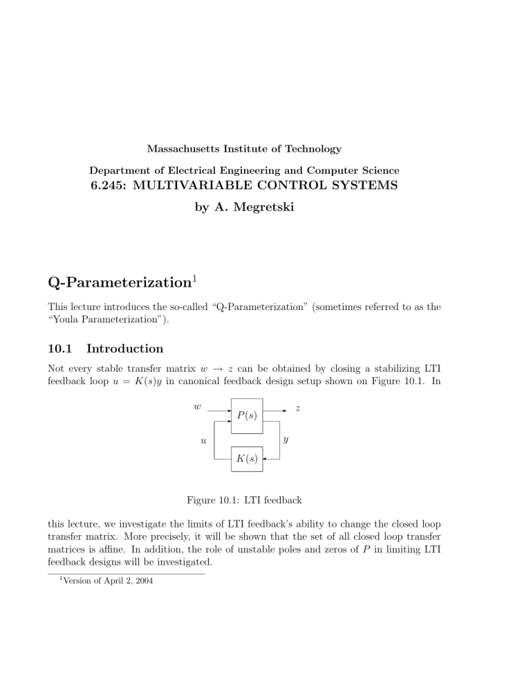
Not every stable transfer matrix w � z can be obtained by closing a stabilizing LTI feedback loop u = K ( s ) y in canonical feedback design setup shown on Figure 10.1.
In w
P ( s ) z u y
K ( s )
�
Figure 10.1: LTI feedback this lecture, we investigate the limits of LTI feedback’s ability to change the closed loop transfer matrix.
More precisely, it will be shown that the set of all closed loop transfer matrices is affine.
In addition, the role of unstable poles and zeros of P in limiting LTI feedback designs will be investigated.
1 Version of April 2, 2004

2
Q-parameterization gives a very simple affine description of the set of all achievable closed loop transfer matrices as function of the so-called “Q” parameter Q = Q ( s ), which is an arbitrary stable proper transfer matrix of size m × k , where m is the total number of actuator inputs, and k is the total number of sensors in the system.
For design purposes, the result is extremely important: instead of thinking in terms of the controller transfer matrix K = K ( s ), one will be much better off by designing Q ( s ).
10.2
The Q-parameterization theorem
We consider LTI systems P from Figure 10.1
(where u and y are vectors of size m and k respectively) given in the state space format
�
P ( s ) :=
⎞
A
C
1
C
2
B
1
D
11
D
21
� B
2
D
12 �
.
0
(10.1)
An LTI feedback controller u = − Kx , where
K :=
⎠ A f
C f
B f
D f
⎛
(10.2) is said to stabilize the feedback system if all eigenvalues of the matrix
�
A cl
=
⎝ A + B
2
D f
C
2
B f
C
2
B
2
C f
A f
(10.3) have negative real part.
Let T = T ( s ) be the transfer matrix of the resulting closed loop system with input w and output z :
�
T :=
⎞
A + B
2
D f
C
2
B f
C
2
C
1
+ D
12
D f
C
2
B
2
C f
A f
D
12
C f
B
1
+ B
2
D f
D
21
B f
D
21
D
11
+ D
12
D f
D
21
�
�
.
(10.4)
Note that the description of T given in (10.4) is very inconvenient for design purposes, because the design parameters A f
, B f
, C f
, D f enter the transfer matrix defined by (10.4) in a very non-linear way, and are themselves constrained nonlinearly by the condition that
A cl in (10.3) must be a Hurwitz parameterization of all T = T ( s ).
matrix.
The following result gives a much more useful

3
Theorem 10.1
Let F, L be constant gains such that matrices A + B
2
F and A + LC
2 are Hurwitz.
Then a given transfer matrix T = T ( s ) can be made equal to the transfer matrix of the closed loop system (10.4) by an appropriate selection of a stabilizing feedback controller (10.2) if and only if
T ( s ) = T
0
( s ) + T
1
( s ) Q ( s ) T
2
( s ) (10.5) for some stable proper rational transfer matrix Q = Q ( s ) , where T
0
, T
1
, T
2 matrices of systems are the transfer
T
0
=
� A
⎞
− LC
2
B
2
F
A + B
2
F + LC
2
C
1
D
12
F
� B
1
− LD
21 �
,
D
11
(10.6)
T
1
T
2
=
=
⎠ A + B
2
F
C
1
+ D
12
F
⎠ A + LC
2
C
2
B
1
D
+ LD
21
D
B
12
21
2
⎛
,
⎛
.
(10.7)
(10.8)
Moreover, T ( s ) can be achieved by using a strictly proper stabilizing controller if and only if representation (10.5) with a stable strictly proper rational Q is possible.
Theorem 10.1
is a remarkable result, which, in particular, ensures that any convex feedback optimization problem formulated in terms of the closed loop transfer matrices can be solved relatively easily.
In (10.5), T
0 and the structure of T
1
, T
2 represents some admissible closed loop design, imposes limitations on the closed loop transfer matrix.
10.3
Derivation of Youla parameterization
Let F, L be defined as in Theorem 10.1, i.e.
A + B
2
F and A + LC
2
For any u ( · ) let ˆ be defined by are Hurwitz matrices.
Then for e = x − ˆ we have e ˙ = ( A + LC
2
) e + ( B
1
+ LD
21
) w.
Let
ˆ˙ = A x + B
2 u + L ( C
2
ˆ − y ) .
� = y − C
2
ˆ = C
2 e + D
21 w.

4
Note that � is the output of system T
2 be re-written in the form with input w .
Now the equations for ˆ x f
, u can
˙ˆ = ( A + B
2
D f
C
2
)ˆ + B
2
C f x f
+ ( B
2
D f
− L ) �, x f
= B f
C
2
ˆ + A f x f
+ B f
�, u − F ˆ = ( D f
C
2
− K )ˆ + C f x f
+ D f
�.
Hence, for a stabilizing controller (10.2), u − F ˆ is the output of the stable system
Q =
�
⎞
� D f
C
2
A
− cl
F C f
�
⎝ B
2
D
B f f
D f
− L � �
� with input � , where A cl is defined
F ˆ w, e, z can be written as by (10.3).
Since, in addition, the equations for x, u − x ˙ = ( A + B
2
F ) x + B
2
( u − F ˆ ) + ( B
1 w − B
2
F e ) z = ( C
1
+ D
12
F ) x + D
12
( u − F ˆ ) + ( D
11 w − D
12
F e ) , z equals the output of T
1 with input u − F ˆ plus the output of T
0 with input w .
This proves that the closed loop transfer matrix from w to z has the form (10.5) with some stable Q .
Conversely, if Q is stable, using u which is a sum of F ˆ and the output of Q with input � defines a stabilizin feedback controller u = Ky .
Figure 10.2
gives a simple interpretation of Q-parameterization: in order to describe a general form of a stabilizing LTI controller, one has to find a special stabilizing controller first, then use a copy of the stabilized system as an estimator of the sensor output, and feed a stable LTI transformation Q = Q ( s ) of the difference between the actual and the estimated sensor values back into the control input.
10.4
Open loop zeros
The restrictions on the closed loop transfer function imposed by the Youla parameteriza­ tion can be understood in terms of the so-called open loop zeros .
To define zeros of MIMO systems, consider state space models x
1
= ax
1
+ bu
1
, y
1
= cx
1
+ du
1
, where the dimensions of x
1
, u
1 matrix and y
1 are n, m and k respectively.
Consider the complex
⎝ �
M ( s ) = a − sI b c d

5 w
P
�
�
K
0
�
0
�
�
P
K
0
� z
−
�
�
Q
Figure 10.2: Youla parameterization where s � C is a scalar complex variable.
The system is said to have a right zero at a point s if ker M ( s ) = { 0 } , i.e.
if M ( s ) is not left invertible, or, equivalently, if there exists a non-zero pair ( X
1
, U
1
) of complex vectors such that sX
1
= aX
1
+ bU
1
, 0 = cX
1
+ dU
1
.
Similarly, the system is said to have a left zero at s if the range of M ( s ) is not the whole vector space C n + k
, i.e.
if M ( s ) is not right invertible, or, equivalently, if there exists a non-zero pair ( p
1
, q
1
) of complex vectors such that sp
1
= p
1 a + q
1 c, 0 = p
1 b + q
1 d.
As it can be seen from the formulae for T
1 and T
2
, the restrictions transfer matrix are caused by the unstable right zeros of the system on the closed loop
˙ = Ax + B
1 w, y = C
2 x + D
21 w, (10.9) and by the unstable left zeros of the system
˙ = Ax + B
2 u, z = C
1 x + D
12 u.
(10.10)
It can be seen immediately that the right zeros of (10.9) cause problems by obstructing the observation process , while the left zeros of (10.10) describe problems which a control action will expecrience even in the case of a complete knowledge of w and x .

6
10.5
Time-Domain Q-Parameterization
The following statement re-states Theorem 10.1
in a time-domain format.
Theorem 10.2
A matrix-valued function Z = Z ( t ) is a closed-loop impulse response from w to z generated in the closed loop system (10.4) by an appropriate selection of a stabilizing feedback controller (10.2) if and only if there exists a function Q = Q ( t ) , elements of which are finite linear combinations of Dirac deltas � = � ( t ) and generalized one-sided exponents t k e st u ( t ) with Re( s ) < 0 , such that
Z ( t ) = ( C + D
12
F ) X ( t ) + D
12
V ( t ) + D
11
� ( t ) , where
V ( t ) = �( t )( B
1
+ LD
21
) + Q ( t ) D
21
,
˙ t ) = �( t )( A + LC
2
) + Q ( t ) C
2
,
X t ) = ( A + B
2
F ) X ( t ) + B
2
V ( t ) + B
1
� ( t ) , and X ( · ) , �( · ) are zero for t < 0 .