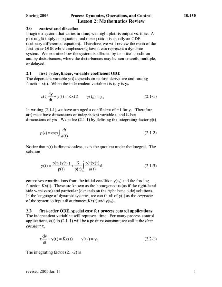
Spring 2006
Process Dynamics, Operations, and Control
10.450
Lesson 2: Mathematics Review
2.0
context and direction
Imagine a system that varies in time; we might plot its output vs. time. A
plot might imply an equation, and the equation is usually an ODE
(ordinary differential equation). Therefore, we will review the math of the
first-order ODE while emphasizing how it can represent a dynamic
system. We examine how the system is affected by its initial condition
and by disturbances, where the disturbances may be non-smooth, multiple,
or delayed.
2.1
first-order, linear, variable-coefficient ODE
The dependent variable y(t) depends on its first derivative and forcing
function x(t). When the independent variable t is t0, y is y0.
a (t)
dy
+ y( t ) = Kx ( t )
dt
y( t 0 ) = y 0
(2.1-1)
In writing (2.1-1) we have arranged a coefficient of +1 for y. Therefore
a(t) must have dimensions of independent variable t, and K has
dimensions of y/x. We solve (2.1-1) by defining the integrating factor p(t)
p(t ) = exp ∫
dt
a(t )
(2.1-2)
Notice that p(t) is dimensionless, as is the quotient under the integral. The
solution
t
p( t 0 ) y( t 0 ) K p( t ) x ( t )
y( t ) =
+
dt
p( t )
p( t ) t∫0 a ( t )
(2.1-3)
comprises contributions from the initial condition y(t0) and the forcing
function Kx(t). These are known as the homogeneous (as if the right-hand
side were zero) and particular (depends on the right-hand side) solutions.
In the language of dynamic systems, we can think of y(t) as the response
of the system to input disturbances Kx(t) and y(t0).
2.2
first-order ODE, special case for process control applications
The independent variable t will represent time. For many process control
applications, a(t) in (2.1-1) will be a positive constant; we call it the time
constant τ.
τ
dy
+ y( t ) = Kx ( t )
dt
y( t 0 ) = y 0
(2.2-1)
The integrating factor (2.1-2) is
revised 2005 Jan 11
1
Spring 2006
Process Dynamics, Operations, and Control
10.450
Lesson 2: Mathematics Review
p( t ) = exp ∫
t
dt
=e τ
τ
(2.2-2)
and the solution (2.1-3) becomes
y( t ) = y 0 e
−( t − t 0 )
t
τ
+
K −t τ t τ
e ∫ e x ( t )dt
τ
t0
(2.2-3)
The initial condition affects the system response from the beginning, but
its effect decays to zero according to the magnitude of the time constant larger time constants represent slower decay. If not further disturbed by
some x(t), the first order system reaches equilibrium at zero.
However, most practical systems are disturbed. K is a property of the
system, called the gain. By its magnitude and sign, the gain influences
how strongly y responds to x. The form of the response depends on the
nature of the disturbance.
Example: suppose x is a unit step function at time t1. Before we proceed
formally, let us think intuitively. From (2.2-3) we expect the response y to
decay toward zero from IC y0. At time t1, the system will respond to being
hit with a step disturbance. After a long time, there will be no memory of
the initial condition, and the system will respond only to the disturbance
input. Because this is constant after the step, we guess that the response
will also become constant.
Now the math: from (2.2-3)
y( t ) = y 0 e
= y 0e
−( t − t 0 )
−( t − t 0 )
t
K −t τ t τ
e ∫ e U( t − t1 )dt
τ
t0
τ
+
τ
− ( t − t1 )
⎛
τ ⎞
+ KU( t − t1 )⎜1 − e
⎟
⎠
⎝
(2.2-4)
Figure 2.2-1 shows the solution. Notice that the particular solution makes
no contribution before time t1. The initial condition decays, and with no
disturbance would continue to zero. At t1, however, the system responds
to the step disturbance, approaching constant value K as time becomes
large. This immediate response, followed by asymptotic approach to the
new steady state, is characteristic of first-order systems. Because the
response does not track the step input faithfully, the response is said to lag
behind the input; the first-order system is sometimes called a first-order
lag.
revised 2005 Jan 11
2
Spring 2006
Process Dynamics, Operations, and Control
10.450
disturbance
Lesson 2: Mathematics Review
1
0.5
0
2.5
0
1
2
3
4
5
6
0t 0
1
2t 1
3
4
5
6
response
2y 0
1.5
1K
0.5
0
time
Figure 2.2-1 first-order response to initial condition and step
disturbance
2.3
piecewise integration of non-smooth disturbances
The solution (2.2-3) is applied over succeeding time intervals, each
featuring an initial condition (from the preceding interval) and disturbance
input.
t
−(t − t 0 )
⎧
K −t τ t τ
τ
+ e ∫ e x ( t )dt
⎪ y( t 0 )e
τ
t0
⎪
⎪
t
− ( t − t1 )
t
K −t
⎪
τ
+ e τ ∫ e τ x ( t )dt
y ( t ) = ⎨ y ( t 1 )e
τ
t1
⎪
⎪etc.
⎪
⎪⎩
t 0 < t < t1
t1 < t < t 2
(2.3-1)
Example: suppose
revised 2005 Jan 11
3
Spring 2006
Process Dynamics, Operations, and Control
10.450
Lesson 2: Mathematics Review
dy
y ( 0) = 0
+y=x
dt
0 < t <1
⎧0
⎪
x = ⎨2(t − 1) 1 < t < 2
⎪0
2<t
⎩
(2.3-2)
In this problem, variables t, x, and y should be presumed to have
appropriate, if unstated, units; in these units, both gain and time constant
are of magnitude 1. From (2.3-1),
⎧0
⎪
y( t ) = ⎨2 t − 2 + e −(t −1)
⎪2e −1e −( t − 2 )
⎩
(
)
0 < t <1
1< t < 2
(2.3-3)
2<t
With a zero initial condition and no disturbance, the system remains at
equilibrium until the ramp disturbance begins at t = 1. Then the output
immediately rises in response, lagging behind the linear ramp. At t = 2,
the disturbance ceases, and the output decays back toward equilibrium.
revised 2005 Jan 11
4
Spring 2006
Process Dynamics, Operations, and Control
10.450
Lesson 2: Mathematics Review
2.5
disturbance
2
1.5
1
0.5
0
0
1
2
3
4
5
6
0
1
2
3
4
5
6
0.8
0.7
response
0.6
0.5
0.4
0.3
0.2
0.1
0
time
2.4
multiple disturbances and superimposition
Systems can have more than one input. Consider a first-order system with
two disturbance functions.
τ
dy
+ y( t ) = K1x 1 ( t ) + K 2 x 2 ( t )
dt
y( t 0 ) = y 0
(2.4-1)
Applying (2.2-3) and distributing the integral across the disturbances, we
find that the effects of the disturbances on y are additive.
y( t ) = y 0 e
−( t − t 0 )
t
τ
+
t
t
K1 − t τ t τ
K −t
e ∫ e x1 ( t )dt + 2 e τ ∫ e τ x 2 ( t )dt (2.4-2)
τ
τ
t0
t0
This additive behavior is a happy characteristic of linear systems. Thus
another way to view problem (2.4-1) is to decompose it into component
problems. That is, define
y = y H + y1 + y 2
revised 2005 Jan 11
(2.4-3)
5
Spring 2006
Process Dynamics, Operations, and Control
10.450
Lesson 2: Mathematics Review
and write (2.4-1) in three equations. We put the initial condition with no
disturbances, and each disturbance with a zero initial condition.
dy H
+ yH (t) = 0
dt
dy
τ 1 + y1 ( t ) = K1x1 ( t )
dt
dy
τ 2 + y 2 (t) = K 2 x 2 (t)
dt
τ
yH (t 0 ) = y0
y1 ( t 0 ) = 0
(2.4-4)
y2 (t 0 ) = 0
Equations and initial conditions (2.4-4) can be summed to recover the
original problem specification (2.4-1). The solutions are
y H (t ) = y 0e
−(t −t 0 )
τ
t
y1 ( t ) =
K1 − t τ t τ
e ∫ e x1 ( t )dt
τ
t0
y 2 (t ) =
K 2 −t τ t τ
e ∫ e x 2 ( t )dt
τ
t0
(2.4-5)
t
and of course these solutions can be added to recover original solution
(2.4-2). Thus we can view the problem of multiple disturbances as a
system responding to the sum of the disturbances, or as the sum of
responses from several identical systems, each responding to a single
disturbance.
Example: consider
3
1 dy 1
+ y = U ( t − 1) − U ( t − 3)
4
4 dt 4
y ( 0) = 2
(2.4-6)
We first place the equation in standard form, in which the coefficient of y
is +1.
dy
+ y = 3U ( t − 1) − 4 U ( t − 3)
dt
y ( 0) = 2
(2.4-7)
Equation (2.4-7) shows us that the time constant is 1, and that the system
responds to the first disturbance with a gain of 3, and to the second with a
gain of -4. The solution is
y = 2e − t + 3U( t − 1)(1 − e − ( t −1) ) − 4U( t − 3)(1 − e − ( t −3) )
revised 2005 Jan 11
(2.4-8)
6
Spring 2006
Process Dynamics, Operations, and Control
10.450
Lesson 2: Mathematics Review
In Figure 2.4-1, the individual solution components are plotted as solid
traces; their sum, which is the system response, is a dashed trace. Notice
how the first-order lag responds to each new disturbance as it occurs.
disturbances
1
0.5
0
0
2
4
6
8
0
2
4
6
8
4
3
2
response
1
0
-1
-2
-3
-4
-5
time
Figure 2.4-1 first-order response to multiple disturbances
Writing the step functions explicitly in solution (2.4-8) emphasizes that
particular disturbances do not influence the solution until the time of their
occurrence. For example, if they were omitted, some deceptively correct
but inappropriate rearrangement would lead to errors.
(
) (
y = 2e − t + 3 1 − e − ( t −1) − 4 1 − e − ( t −3)
= 2e − t + 3 − 3e −( t −1) − 4 + 4e −( t −3)
)
(do not do this!)
(2.4-9)
= −1 + 2e − t − 3e −( t −1) + 4e −( t −3)
This notation at least implies that two of the exponential functions have
delayed onsets. However, further correct-but-inappropriate rearrangement
makes things even worse.
revised 2005 Jan 11
7
Spring 2006
Process Dynamics, Operations, and Control
10.450
Lesson 2: Mathematics Review
y = −1 + 2e − t − 3e − ( t −1) + 4e − ( t −3)
= −1 + 2e − t − 3e1e − t + 4e 3e − t
(
)
= −1 + 2 − 3e + 4e e
1
3
(do not do this!)
(2.4-10)
−t
The incorrect solutions are plotted with (2.4-8) in Figure 2.4-2. Equation
(2.4-9) has become discontinuous - the response takes non-physical leaps
at the onset of each new disturbance. Equation (2.4-10) has lost all
dependence on the disturbances and decays from a non-physical initial
condition. Even with the mistakes, both incorrect solutions lead to the
correct long-term condition.
20
response
15
10
5
0
-5
0
2
4
6
8
time
solution
eq 2.4.9
eq 2.4.10
Figure 2.4-2 comparison of correct and incorrect solutions
2.5
delayed response to disturbances
Consider a system that reacts to a disturbance, but only after some
intervening time interval θ has passed. That is
τ
dy
+ y( t ) = Kx ( t − θ)
dt
y( t 0 ) = y 0
(2.5-1)
Equation (2.5-1) shows the dependence of y, at any time t, on the value of
x at earlier time t - θ. The solution is written directly from (2.2-3).
y( t ) = y 0 e
−( t − t 0 )
t
τ
+
K −t τ t τ
e ∫ e x ( t − θ)dt
τ
t0
(2.5-2)
We must integrate the disturbance considering the time delay. Take as an
example a disturbance x(t) occurring at time t1. The plot shows the
revised 2005 Jan 11
8
Spring 2006
Process Dynamics, Operations, and Control
10.450
Lesson 2: Mathematics Review
disturbance, as well as the disturbance as the system experiences it, which
begins at time t1 + θ. We could express this disturbance-as-experienced as
some new function x1(t), occurring at time t1 + θ.
disturbance as
experienced by
system
disturbance
as it occurs
x(t)
t0
x(t - θ) = x1(t)
t1 + θ
t1
t
x(ξ)
t0 - θ
t1 - θ
t1
ξ
Alternatively, we could define a new time variable
ξ = t−θ
(2.5-3)
and write the input as x(ξ). The integral in (2.5-2) becomes, then,
t
t
t
t
∫ e x (t − θ)dt = ∫ e x1 (t )dt =
τ
t0
τ
t0
ξ
∫e
ξ+θ
τ
x (ξ)dξ
(2.5-4)
t 0 −θ
Therefore, solution (2.5-2) becomes
y( t ) = y 0 e
−( t − t 0 )
ξ
τ
ξ
K −t θ
+ e τ e τ ∫ e τ x (ξ)dξ
τ
t 0 −θ
(2.5-5)
Example: consider a step disturbance at time t = 2 that affects the system
3 time units later.
dy
+ y = x ( t − 3)
dt
x ( t ) = U( t − 2)
y(0) = 0
(2.5-6)
Using (2.5-5)
revised 2005 Jan 11
9
Spring 2006
Process Dynamics, Operations, and Control
10.450
Lesson 2: Mathematics Review
ξ
y = e − t e 3 ∫ e ξ U(ξ − 2)dξ
0 −3
ξ
⎡2 ξ
⎤
= e e ⎢ ∫ e U(ξ − 2)dξ + ∫ e ξ U(ξ − 2)dξ⎥
2
⎣⎢0−3
⎦⎥
−t
3
= e − t e 3 ⎡ U (ξ − 2)e ξ ⎤
⎢⎣
2⎥
⎦
− t 3 t −3
= U( t − 3 − 2)e e e − e 2
(2.5-7)
ξ
[
= U( t − 5)[1 − e
[
= U( t − 5) e t −3− t +3 − e 2− t +3
− ( t −5 )
]
]
]
Figure 2.5-1 shows that a typical first-order lag step response occurs 3
time units after being disturbed at t = 2.
disturbances
1
0.5
0
0
2
4
6
8
10
0
2
4
6
8
10
1
response
0.8
0.6
0.4
0.2
0
time
Figure 2.5-1 step response of first order system with dead time
The time delay in responding to a disturbance is often called dead time.
Dead time is different from lag. Lag occurs because of the combination of
y and its derivative on the left-hand side of the equation. Dead time
revised 2005 Jan 11
10
Spring 2006
Process Dynamics, Operations, and Control
10.450
Lesson 2: Mathematics Review
occurs because of a time delay in processing a disturbance on the righthand side.
2.6
conclusion
Please become comfortable with handling ODEs. View them as systems;
identify their inputs and outputs, their gains and time parameters.
revised 2005 Jan 11
11