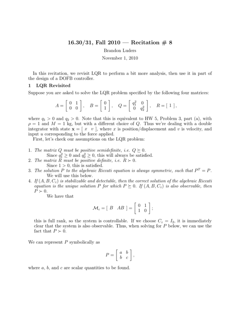
16.30/31, Fall 2010 — Recitation # 8
Brandon Luders
November 1, 2010
In this recitation, we revisit LQR to perform a bit more analysis, then use it in part of
the design of a DOFB controller.
1
LQR Revisited
Suppose you are asked to solve the LQR problem specified by the following four matrices:
�
�
� �
� 2
�
0 1
0
q
1 0
A =
,
B
=
,
Q =
,
R = [ 1 ] ,
0 0
1
0 q
22
where q1 > 0 and q2 > 0. Note that this is equivalent to HW 5, Problem 3, part (a), with
ρ = 1 and M = 1 kg, but with a different choice of Q. Thus we’re dealing with a double
integrator with state x = [ x v ], where x is position/displacement and v is velocity, and
input u corresponding to the force applied.
First, let’s check our assumptions on the LQR problem:
1. The matrix Q must be positive semidefinite, i.e. Q � 0.
Since q
12 ≥ 0 and q
22 ≥ 0, this will always be satisfied.
2. The matrix R must be positive definite, i.e. R � 0.
Since 1 > 0, this is satisfied.
3. The solution P to the algebraic Riccati equation is always symmetric, such that P T = P .
We will use this below.
4. If (A, B, Cz ) is stabilizable and detectable, then the correct solution of the algebraic Riccati
equation is the unique solution P for which P � 0. If (A, B, Cz ) is also observable, then
P � 0.
We have that
�
�
0 1
Mc = [ B AB ] =
;
1 0
this is full rank, so the system is controllable. If we choose Cz = I2 , it is immediately
clear that the system is also observable. Thus, when solving for P below, we can use the
fact that P � 0.
We can represent P symbolically as
�
P =
a b
b c
�
where a, b, and c are scalar quantities to be found.
,
We now plug everything into the algebraic Riccati equation to solve for P :
0 = AT P + P A + Q − P BR−1 B T P
�
��
� �
��
� � 2
�
0 0
a b
a b
0 1
q1 0
=
+
+
1 0
b c
b c
0 0
0 q22
�
�� �
�
�
a b
0 1
a b
−
[ 0 1 ]
b c
1 1
b c
�
� �
� � 2
�
0 0
0 a
q1 0
=
+
+
a b
0 b
0 q22
�
��
��
�
a b
0 0
a b
−
b c
0 1
b c
� 2
� �
��
�
q1
a
a b
0 0
=
−
b c
b c
a 2b + q22
� 2
� � 2
�
q1
a
b bc
=
−
a 2b + q22
bc c2
� 2
�
q 1 − b2
a − bc
=
.
a − bc 2b + q22 − c2
Since this equation is always symmetric, this yields three distinct equations with three un­
knowns (a, b, c):
�
q12 − b2 = 0
a − bc = 0
2b + q22 − c2 = 0
The first equation is only a function of b, so we can quickly solve it to find that b = ±q1 .
Plug this into the third equation:
±2q1 + q22 − c2 = 0
⇒ c2 = q22 ± 2q1
�
⇒ c = ± q22 ± 2q1
One consquence of Sylvester’s criterion is that for P to be positive definite,
all of its diagonal
�
2
elements must be positive; thus we need c > 0, implying that c = q2 ± 2q1 . Finally, plug
b and c into the second equation:
��
�
�
2
a = bc = (±q1 )
q2 ± 2q1 = ±q1 q22 ± 2q1 .
This yields two possible choices for P :
�
� � 2
�
�
�
q1 q2 + 2q1 � q1
−q1 q22 − 2q1 � −q1
P =
or P =
.
q1
q22 + 2q1
−q1
q22 − 2q1
Again by Sylvester’s criterion, since q1 > 0, only the first choice is valid; thus
� � 2
�
q1 q2 + 2q1 � q1
P =
.
q1
q22 + 2q1
2
We now have all we need to find K:
K = R−1 B T P
� � 2
�
1
q1 q2 + 2q1 �
q1
= [ 0 1 ]
1
q1
q
22 + 2q1
�
�
�
= q1
q22 + 2q1 .
We’ve now solved for the LQR feedback K, in terms of q1 and q2 . An important part of
analysis for LQR problems is considering how the control would vary if the LQR weights Q
and R are modified. For example, for just this simple double integrator we can draw many
conclusions:
1. As both q1 and q2 increase, K → [ ∞ ∞ ], reflecting that the relative weight on control
effort is shrinking.
2. Conversely, as q1 and q2 → 0, K → [ 0 0 ], since we have that Q → 0 but still R = 1.
3. Suppose q2 is fixed. As q1 increases, both gains increase, but the gain on displacement (the
first gain) increases more quickly. In this case, there is a larger penalty on displacement
than velocity, so the controller adjusts to cancel displacement more quickly.
4. Suppose q2 is fixed. As q1 → 0, K → [ 0 q2 ]. This is what we call a velocity controller ­
the controller ignores displacement, and merely tries to regulate the velocity back to zero.
5. Suppose q1 is fixed. As q2 increases, only the velocity gain (the second gain) increases.
(This is similar to #4 in a relative sense.)
�
�
√
2q1 .
Contrast this with #4 - whereas
6. Suppose q1 is fixed. As q2 →
0, K →
q1
velocity can be controlled with a single non-zero gain, both gains are used to regulate the
position back to 0.
Moving forward, we choose q1 = 8 and q2 = 0, such that K = [ 8 4 ]. Let’s compute the
closed-loop poles:
�
� � �
0 1
0
A − BK =
−
[ 8 4 ]
0 0
1
�
�
0
1
=
−8 −4
�
�
� s −1 �
�
det(sI − (A − BK)) =
��
8
s + 4 �
= s2 + 4s + 8
�
√
−4 ± 42 − 4(8)
−4 ± −16
s =
=
=
−2 ± 2j
2
2
2
DOFB Compensators
Now, consider the system
ẋ = Ax + Bu,
y = Cx,
where A and B are as given in the previous section and C = [ 1 0 ]. This C implies that
for this double integrator, we can only measure the displacement, not the velocity. Our
objective is to regulate both the system displacement and velocity to 0.
3
Clearly, full-state feedback u = −Kx is not possible for this problem, as only the displace­
ment can be measured. Likewise, it should make sense that feedback of the form u = −Ky
is not helpful - it will always apply the same control for the same displacement, regardless of
whether the system is stationary or has a huge velocity. Thus, we will need to construct an
estimator to develop a system state estimate x̂, then apply feedback of the form u = −Kx̂.
For K, we’ll use the LQR controller we designed in the previous section.
The closed-loop estimator will take the form
x̂˙ = (A − LC)x̂ + Bu + Ly,
ŷ = Cx̂,
where L is a gain we can choose to place the closed-loop estimator poles appropriately.
We know that we can place the eigenvalues of A − LC arbitrarily if (A, C) is observable,
something we can easily check:
�
� �
�
C
1 0
Mo =
=
.
CA
0 1
Since this is clearly full rank, the system is observable.
We are thus free to place the estimator poles anywhere. Using the rule of thumb, we
choose poles whose real part is twice those of the regulator poles, i.e. 2(−2) ± 2j = −4 ± 2j.
The easiest way to pick L is to simply use the dual of Ackermann’s formula, which gives us
the estimator gain yielding the desired closed-loop poles:
Φd (s) = (s + 4 − 2j)(s + 4 + 2j) = s2 + 8s + 20
I2 � 0 �
�
−
1
L = Φd (A) �
M�o
1
�
�� �
0
0
2
= �
A�
+ 8A + 20I2
1
��
� �
�� � �
0 8
20 0
0
=
+
0 0
0 20
1
�
�� � �
�
20 8
0
8
=
=
.
0 20
1
20
With K and L, we now have everything we need to form the dynamic output feedback
(DOFB) compensator necessary to regulate this system:
ẋc = Ac xc + Bc y
u = −Cc xc
Ac = A − BK − LC
�
� � �
�
�
0 1
0
8
=
−
[ 8 4 ]−
[ 1 0 ]
0 0
1
20
�
� �
� �
� �
�
0 1
0
0
−8 0
−8 1
=
+
+
=
0 0
−8 −4
−20 0
−28 −4
�
�
8
Bc = L =
20
Cc = K = [ 8 4 ]
4
We could go ahead and form the closed-loop state space model, but we already know from
the separation principle that its poles will be the union of the regulator and estimator poles
we have already selected, i.e. −4 ± 2j and −2 ± 2j.
To finish things off, let’s perform some analysis of this controller. Write the transfer
functions for the plant and controller:
Y (s)
= C(sI − A)−1 B
U (s)
�
�−1 � �
1
s −1
0
=[ 1 0 ]
= 2
0 s
1
s
U (s)
Gc (s) =
= Cc (sI − Ac )−1 Bc
E(s)
�
�−1 �
�
s + 8 −1
8
=[ 8 4 ]
28 s + 4
20
�
��
�
1
s+4
1
8
= 2
[ 8 4 ]
−28 s + 8
20
s + 12s + 60
�
�
1
144s − 160
8s + 52
= 2
[ 8 4 ]
= 2
20s − 64
s + 12s + 60
s + 12s + 60
√
This controller has a zero at −10/9 and poles at −6 ± j 24 - but why? This is not a type of
controller (one zero, two complex poles) we considered classically. Yet the root locus shows
that this controller places our four closed-loop poles exactly where we wanted them to be:
Gp (s) =
The zero sucks the two open-loop poles at the origin back into the LHP enough to reach
the desired locations, before they head along the asymptotes back into the RHP. Also, note
from the Bode plot that the controller does a nice job of adding phase (about 37◦ ) right
where it’s needed, at crossover.
5
MIT OpenCourseWare
http://ocw.mit.edu
16.30 / 16.31 Feedback Control Systems
Fall 2010
For information about citing these materials or our Terms of Use, visit: http://ocw.mit.edu/terms.