IV. Perturbative Renormalization Group
IV.A Expectation Values in the Gaussian Model
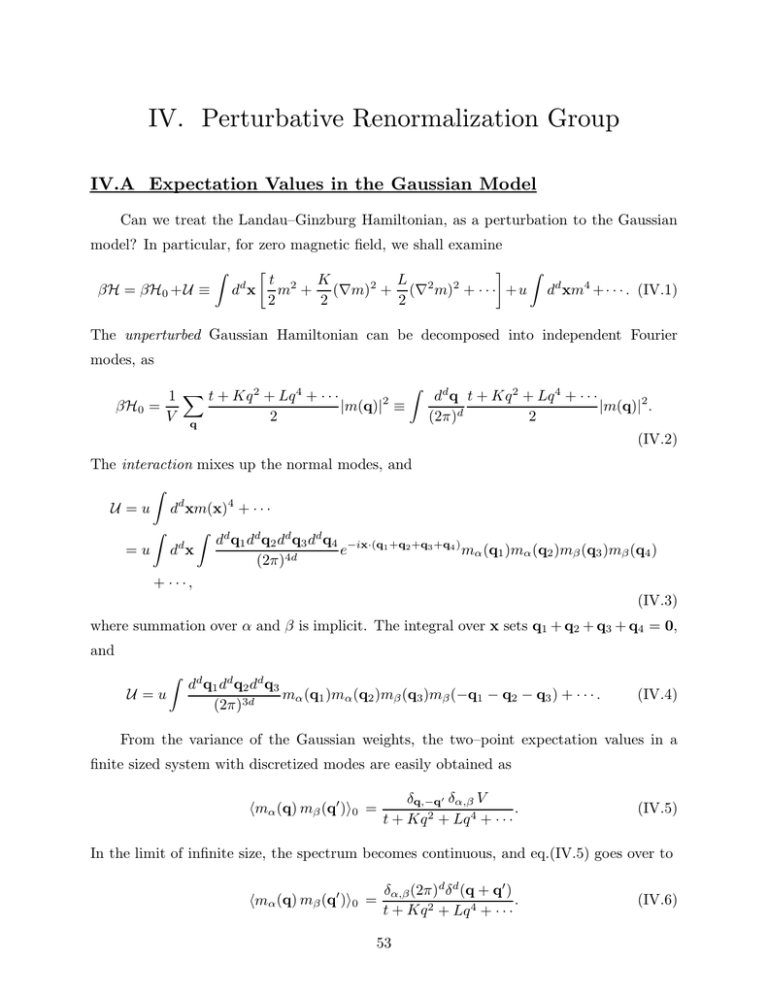
Can we treat the Landau–Ginzburg Hamiltonian, as a perturbation to the Gaussian
model? In particular, for zero magnetic field, we shall examine
βH = βH0 +U ≡
Z
Z
L 2 2
t 2 K
2
d x m + (∇m) + (∇ m) + · · · +u dd xm4 +· · · . (IV.1)
2
2
2
d
The unperturbed Gaussian Hamiltonian can be decomposed into independent Fourier
modes, as
Z
1 X t + Kq 2 + Lq 4 + · · ·
dd q t + Kq 2 + Lq 4 + · · ·
2
βH0 =
|m(q)| ≡
|m(q)|2 .
2
V q
2
(2π)d
(IV.2)
The interaction mixes up the normal modes, and
Z
dd xm(x)4 + · · ·
Z
Z d
d q1 dd q2 dd q3 dd q4 −ix·(q1 +q2 +q3 +q4 )
d
=u d x
e
mα (q1 )mα (q2 )mβ (q3 )mβ (q4 )
(2π )4d
U =u
+ ···,
(IV.3)
where summation over α and β is implicit. The integral over x sets q1 + q2 + q3 + q4 = 0,
and
U =u
Z
dd q1 dd q2 dd q3
mα (q1 )mα (q2 )mβ (q3 )mβ (−q1 − q2 − q3 ) + · · · .
(2π)3d
(IV.4)
From the variance of the Gaussian weights, the two–point expectation values in a
finite sized system with discretized modes are easily obtained as
hmα (q) mβ (q′ )i0 =
δq,−q′ δα,β V
.
t + Kq 2 + Lq 4 + · · ·
(IV.5)
In the limit of infinite size, the spectrum becomes continuous, and eq.(IV.5) goes over to
hmα (q) mβ (q′ )i0 =
δα,β (2π)d δ d (q + q′ )
.
t + Kq 2 + Lq 4 + · · ·
53
(IV.6)
The subscript 0 is used to indicate that the expectation values are taken with respect to
the unperturbed (Gaussian) Hamiltonian. Expectation values involving any product of
m’s can be obtained starting from the identity


*
"
#+
X
X ai aj
hmi mj i0  ,
= exp 
(IV.7)
exp
ai mi
2
i
i,j
0
which is valid for any set of Gaussian distributed variables {mi }. (This is easily seen by
‘completing the square.’) Expanding both sides of the equation in powers of {ai } leads to
ai aj
ai aj ak
ai aj ak al
hmi mj i0 +
hmi mj mk i0 +
hmi mj mk mk i0 + · · · =
2
6
24
ai aj ak al
ai a j
hmi mj i0 +
(hmi mj i0 hmk ml i0 + hmi mk i0 hmj ml i0 + hmi mk i0 hmj ml i0 )
1+
2
24
+ ···.
(IV.8)
Matching powers of {ai } on the two sides of the above equation gives
* ℓ
+
(
0
for ℓ odd
Y
mi
=
.
(IV.9)
i=1
sum over all pairwise contractions for ℓ even
0
1 + ai hmi i0 +
This result is known as Wick’s theorem; and for example,
hmi mj mk ml i0 = hmi mj i0 hmk ml i0 + hmi mk i0 hmj ml i0 + hmi mk i0 hmj ml i0 .
IV.B Expectation values in Perturbation Theory
In the presence of an interaction U, the expectation value of any operator O, is
computed perturbatively as follows:
R
R
Dm
� e−β H0 O[1 − U + U 2 /2 − · · ·]
Dm
� Oe−β H0 −U
hOi = R
= R
Dm
� e−β H0 −U
Dm
� e−β H0 [1 − U + U 2 /2 − · · ·]
(IV.10)
Z0 [hOi0 − hOUi0 + hOU 2 i0 /2 − · · ·]
=
.
Z0 [1 − hUi0 + hU 2 i0 /2 − · · ·]
Inverting the denominator by an expansion in powers of U gives
1 2
1
2
2
hOi = hOi0 − hOUi0 + hOU i0 − · · · 1 + hUi0 + hUi0 − hU i0 − · · ·
2
2
1
hOU 2 i0 − 2hOUi0 hUi0 + 2hOi0 hUi20 − hOi0 hU 2 i0
=hOi0 − (hOUi0 − hOi0 hUi0 ) +
2
∞
n
X
(−1)
c
hOU n i0 .
+··· ≡
n!
n=0
(IV.11)
54
The connected averages are defined as the combination of unperturbed expectation values
appearing at various orders in the expansion. Their significance will become apparent in
diagrammatic representations, and from the following example.
Let us calculate the two point correlation function of the Landau–Ginzburg model
to first order in the parameter u. [In view of their expected irrelevance, we shall ignore
higher order interactions, and also only keep the lowest order Gaussian terms.] Substituting
eq.(IV.4) into eq.(IV.11) yields
Z d
d q1 dd q2 dd q3
′
′
hmα (q) mβ (q )i = hmα (q) mβ (q )i0 − u
(2π)3d
(IV.12)
[hm (q) m (q′ )m (q )m (q )m (q )m (−q − q − q )i −
α
β
i
1
i
2
j
3
j
1
2
3
0
hmα (q) mβ (q′ )i0 hmi (q1 )mi (q2 )mj (q3 )mj (−q1 − q2 − q3 )i0 ] + O(u2 ).
To calculate hOUi0 we need the unperturbed expectation value of the product of six m’s.
This can be evaluated using eq.(IV.9) as the sum of all pair-wise contractions, 15 in all.
Three contractions are obtained by first pairing mα to mβ , and then the remaining four
m’s in U. Clearly these contractions cancel exactly with corresponding ones in hOi0 hUi0 .
The only surviving terms involve contractions that connect O to U. This cancellation
persists at all orders, and hOU n ic0 contains only terms in which all n + 1 operators are
connected by contractions. The remaining 12 pairings in hOUi0 fall into two classes:
(i) 4 pairings involve contracting mα and mβ to m’s with the same index, e.g.
hmα (q) mi (q1 )i0 hmβ (q′ ) mi (q2 )i0 hmj (q3 ) mj (−q1 − q2 − q3 )i0
(IV.13)
δαi δβi δjj (2π)3d δ d (q + q1 ) δ d (q′ + q2 ) δ d (q1 + q2 )
,
2
2
′2
(t + Kq ) (t + Kq ) (t + Kq3 )
where we have used eq.(IV.6). After summing over i and j, and integrating over q1 , q2 ,
and q3 , such terms make a contribution
Z d
nδαβ (2π)d δ d (q + q′ )
1
d q3
−4u
.
(IV.14)
2
2
d
(t + Kq )
(2π) t + Kq32
(ii) 8 pairings involve contracting mα and mβ to m’s with different indices, e.g.
=
hmα (q) mi (q1 )i0 hmβ (q′ ) mj (q3 )i0 hmi (q2 ) mj (−q1 − q2 − q3 )i0
(IV.15)
δαi δβj δij (2π)3d δ d (q + q1 ) δ d (q′ + q3 ) δ d (q1 + q3 )
.
(t + Kq 2 ) (t + Kq ′2 ) (t + Kq22 )
Summing over all indices, and integrating over the momenta leads to an overall contribution
of
Z d
δαβ (2π)d δ d (q + q′ )
d q2
1
−8u
.
(IV.16)
(t + Kq 2 )2
(2π)d t + Kq22
Adding up both contributions, we obtain
Z
dd k
δαβ (2π)d δ d (q + q′ )
1
4u(n + 2)
2
′
hmα (q) mβ (q )i =
+ O(u ) .
1−
t + Kq 2
(2π)d t + Kk 2
t + Kq 2
(IV.17)
=
55
IV.C Diagrammatic Representation of Perturbation Theory
The calculations become more involved at higher orders in perturbation theory. A
diagrammatic representation can be introduced to help keep track of all possible contrac­
Qℓ
tions. To calculate the ℓ–point expectation value h i=1 mαi (qi )i, at pth order in u, proceed
according to the following rules:
(1) Draw ℓ external points labelled by (qi , αi ) corresponding to the coordinates of the re­
quired correlation function. Draw p vertices with 4 legs each, labelled by internal momenta
and indices, e.g. {(k1 , i), (k2 , i), (k3 , j), (k4 , j)}. Since the four legs are not equivalent, the
four point vertex is indicated by two solid branches joined by a dotted line. (The extension
to higher order interactions is straightforward.)
(2) Each point of the graph now corresponds to one factor of mαi (qi ), and the unperturbed
average of the product is computed by Wick’s theorem. This is implemented by joining
all external and internal points pairwise, by lines connecting one point to another, in all
topologically distinct ways (see #5 below).
(3) The algebraic value of each such graph is obtained as follows: (i) A line joining a
pair of points represents the two point average† ; e.g. a connection (q, α) ←→ (q′ , β),
contributes δαα′ (2π)d δ d (q + q′ )/(t + Kq 2 ); (ii) A vertex is represented by a term such as
u(2π)d δ d (k1 + k2 + k3 + k4 ) (the delta-function insures that momentum is conserved).
(4) Integrate over the 4p internal momenta {ki }, and sum over the 2p internal indices.
Note that each closed loop produces a factor of δii = n at this stage.
(5) There is a numerical factor of
(−1)p
× number of different pairings leading to the same topology.
p!
The first contribution comes from the expansion of the exponential; the second merely
states that graphs related by symmetry give the same result, and can be calculated once.
(6) When calculating cumulants, only fully connected diagrams (without disjoint pieces)
need to be included. This is a tremendous simplification.
†
Because of its original formulation in quantum field theory, the line joining two points
is usually called a propagator. In this context, the line represents the world-line of a
particle in time, while the perturbation U is an ‘interaction’ between particles. For the
same reason, the Fourier index is called a ‘momentum.’
56
IV.D Susceptibility
It is no accident that the correction term in eq.(IV.17) is similar in form to the
unperturbed value. This is because the form of the two point correlation function is
constrained by symmetries, as can be seen from
Z
Z
′
′
′
d
hmα (q) mβ (q )i = d x dd x′ eiq·x+iq ·x hmα (x) mβ (x′ )i.
(IV.18)
The two point correlation function in real space must satisfy translation and rotation
symmetry (in the high temperature phase), and hmα (x) mβ (x′ )i = δαβ hm1 (x − x′ ) m1 (0)i.
Transforming to center of mass and relative coordinates, the above integral becomes,
hmα (q) mβ (q′ )i =
Z
′
′
′
′
x + x′ d
d
d
d (x − x′ ) ei(q+q )·(x+x )/2 ei(x−x )·(q−q )/2 δαβ hm1 (x − x′ ) m1 (0)i
2
≡ (2π)d δ d (q + q′ )δαβ S(q),
(IV.19)
where
S(q) = |m1 (q)|
2
=
Z
dd xeiq·x hm1 (x − x′ ) m1 (0)i,
(IV.20)
is the quantity observed in scattering experiments (sec.II.D).
From eq.(IV.17) we obtain
Z
1
4u (n + 2)
dd k
1
2
+ O(u ) .
S(q) =
1−
t + Kq 2
(2π)d t + Kk 2
t + Kq 2
(IV.21)
It is useful to examine the expansion of the inverse quantity
Z
1
dd k
−1
2
+ O(u2 ).
S(q) = t + Kq + 4u(n + 2)
d
(2π) t + Kk 2
(IV.22)
In the high temperature phase, eq.(IV.20) indicates that the q → 0 limit of S(q) is just
the magnetic susceptibility χ. For this reason, S(q) is sometimes denoted by χ(q). From
eq.(IV.22), the inverse susceptibility is given by
Z
1
dd k
−1
+ O(u2 ).
χ (t) = t + 4u(n + 2)
d
(2π) t + Kk 2
(IV.23)
The susceptibility no longer diverges at t = 0, since
−1
χ
(0) = 4u(n+2)
Z
4(n + 2)u Sd
dd k 1
=
d
2
K
(2π)d
(2π) Kk
57
Z
Λ
dk k
0
d−3
4(n + 2)u
=
Kd
K
Λd−2
,
d−2
(IV.24)
is a finite number. This is because in the presence of u the critical temperature is reduced
to a negative value. The modified critical point is obtained by requiring χ−1 (tc ) = 0, and
hence from eq.(IV.23), to order of u,
tc = −4u(n + 2)
Z
1
4u(n + 2)Kd Λd−2
dd k
≈
−
< 0.
(d − 2)K
(2π)d tc + Kk 2
(IV.25)
How does the perturbed susceptibility diverge at the shifted critical point? From
eq.(IV.23),
−1
χ
−1
(t) − χ
dd k
1
1
(tc ) = t − tc + 4u(n + 2)
−
tc + Kk 2
(2π)d t + Kk 2
Z
4u(n + 2)
dd k
1
2
= (t − tc ) 1 −
+ O(u ) .
(2π)d k 2 (k 2 + (t − tc )/K)
K2
(IV.26)
Z
(In going from the first equation to the second, we have changed the position of tc from
one denominator to another. Since tc = O(u), the corrections to such change only appear
at O(u2 ).) The final integral has dimensions of k d−4 . For d > 4 it is dominated by the
largest momenta and scales as Kd Λd−4 . For 2 < d < 4, the integral is convergent at both
p
limits. Its magnitude is therefore set by the momentum scale ξ −1 = (t − tc )/K, which
can be used to make the integrand dimensionless. Hence, in these dimensions,
"
4u(n + 2)
χ−1 (t) = (t − tc ) 1 −
c
K2
K
t − tc
2−d/2
#
+ O(u2 ) ,
(IV.27)
where c is a constant. For d < 4, the correction term at the order of u diverges at the phase
transition, masking the unperturbed singularity of χ with γ = 1. Thus the perturbation
series is inherently inapplicable for describing the divergence of susceptibility in d < 4.
The same situation applies in calculating any other quantity perturbatively. Although,
we start by treating u as the perturbation parameter, it is important to realize that it is
not dimensionless; u/K 2 has dimensions of (length)d−4 . The perturbation series for any
quantity then takes the form X(t, u) = X0 (t)[1 + f (ua4−d /K 2 , uξ 4−d /K 2 )], where f is
a power series. The two length scales a and ξ are available to construct dimensionless
variables. Since ξ diverges close to the critical point, there is an inherent failure of the
perturbation series. The effective (dimensionless) perturbation parameter diverges at tc
and is not small.
58
MIT OpenCourseWare
http://ocw.mit.edu
8.334 Statistical Mechanics II: Statistical Physics of Fields
Spring 2014
For information about citing these materials or our Terms of Use, visit: http://ocw.mit.edu/terms.