14.123 Microeconomic Theory III
Final Exam
March 18, 2010
(80 Minutes)
1. (30 points) This question assesses your understanding of expected utility theory.
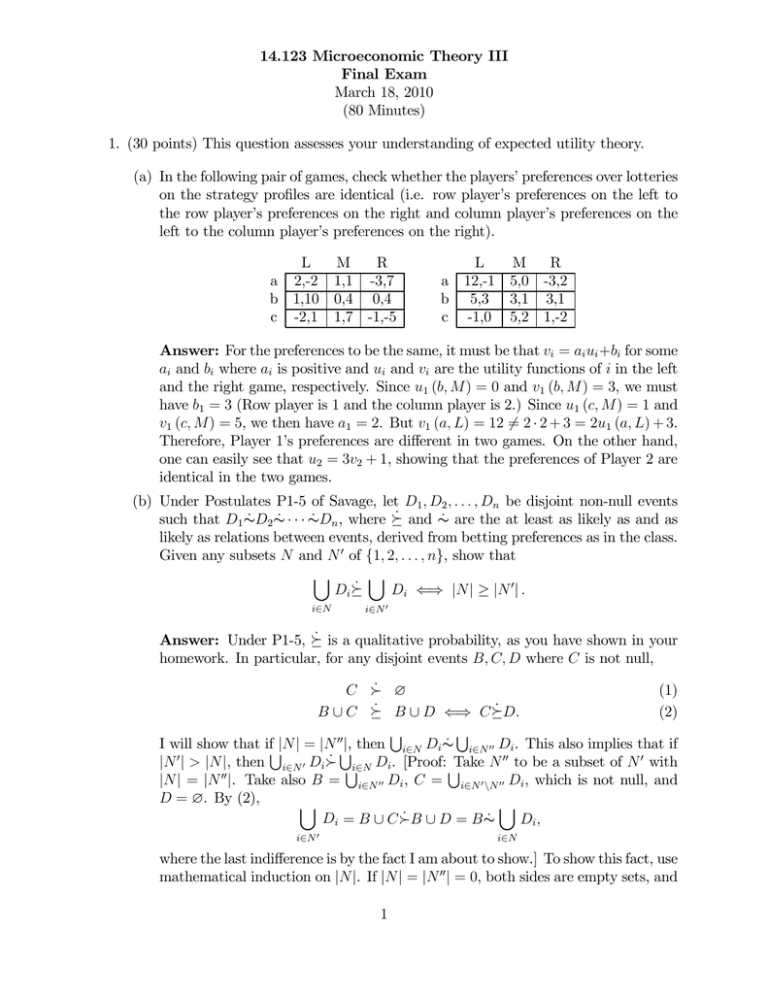
(a) In the following pair of games, check whether the players’ preferences over lotteries
on the strategy profiles are identical (i.e. row player’s preferences on the left to
the row player’s preferences on the right and column player’s preferences on the
left to the column player’s preferences on the right).
L
M
R
a 2,-2 1,1 -3,7
b 1,10 0,4 0,4
c -2,1 1,7 -1,-5
L
M
R
a 12,-1 5,0 -3,2
b 5,3 3,1 3,1
c -1,0 5,2 1,-2
Answer: For the preferences to be the same, it must be that vi = ai ui +bi for some
ai and bi where ai is positive and ui and vi are the utility functions of i in the left
and the right game, respectively. Since u1 (b, M) = 0 and v1 (b, M ) = 3, we must
have b1 = 3 (Row player is 1 and the column player is 2.) Since u1 (c, M) = 1 and
v1 (c, M) = 5, we then have a1 = 2. But v1 (a, L) = 12 6= 2 · 2 + 3 = 2u1 (a, L) + 3.
Therefore, Player 1’s preferences are different in two games. On the other hand,
one can easily see that u2 = 3v2 + 1, showing that the preferences of Player 2 are
identical in the two games.
(b) Under Postulates P1-5 of Savage, let D1 , D2 , . . . , Dn be disjoint non-null events
such that D1 ∼
˙ D2 ∼
˙ ···∼
˙ Dn , where º̇ and ∼
˙ are the at least as likely as and as
likely as relations between events, derived from betting preferences as in the class.
Given any subsets N and N 0 of {1, 2, . . . , n}, show that
[
[
˙
Di º
Di ⇐⇒ |N| ≥ |N 0 | .
i∈N
i∈N 0
Answer: Under P1-5, º̇ is a qualitative probability, as you have shown in your
homework. In particular, for any disjoint events B, C, D where C is not null,
C Â̇ ∅
(1)
B ∪ C º̇ B ∪ D ⇐⇒ Cº̇D.
(2)
S
S
|, then i∈N Di ∼
˙ i∈N 00 Di . This also implies that if
I will show that ifS|N| = |N 00S
|N 0 | > |N|, then i∈N 0 Di Â̇ Si∈N Di . [Proof: STake N 00 to be a subset of N 0 with
|N| = |N 00 |. Take also B = i∈N 00 Di , C = i∈N 0 \N 00 Di , which is not null, and
D = ∅. By (2),
[
[
Di = B ∪ CÂ̇B ∪ D = B∼
˙
Di ,
i∈N 0
i∈N
where the last indifference is by the fact I am about to show.] To show this fact, use
mathematical induction on |N|. If |N| = |N 00 | = 0, both sides are empty sets, and
1
indifference is true. Suppose that the indifference holds for |N| = |N 00 | = m, and
consider N, N 00 with |N| = |N 00 | = m + 1. Let M = N\ {i∗ } and M 00 = N 00 \ {j ∗ }
for some i∗ ∈ N, j ∗ ∈ N 00 . Clearly, |M| = |M 00 | = m, and by inductive hypothesis,
[
[
Di ∼
˙
Di .
(3)
i∈M 00
i∈M
Then,
[
i∈N
Di =
Ã
[
i∈M
Di
!
∪ Di∗ ∼
˙
Ã
[
i∈M
Di
!
∪ Dj ∗ ∼
˙
Ã
[
Di
i∈M 00
!
∪ Dj ∗ =
[
Di ,
i∈N 00
˙ Dj ∗ , and the
where the first indifference is by (2) and the assumption that Di∗ ∼
second indifference is by (2) and (3).
2. (30 points) Consider an expected profit maximizing monopolist who faces an uncertain
demand. He supplies q units of goods at zero cost and sells it at price θ − q, where θ
is unknown. [The price and the supply level can be negative.]
(a) Assuming that θ ∼ N (y, σ 2 ), compute the monopolist’s optimal supply q and his
expected profit under the optimal supply.
Answer: The expected payoff of the monopolist is
E [u] = q (E [θ] − q) = q (y − q) .
Hence, the optimal q is
q ∗ = y/2.
Thus, the payoff under optimal q ∗ is
U (y) = y 2 /4.
(b) Suppose that, through market research, the monopolist can learn about θ. In
particular, by investing c2 , he can learn the value of a random variable Y before
choosing his supply q, such that θ = X + Y , X ∼ N (0, 1 − c) and Y ∼ N (0, c).
How much should the monopolist invest? [Note that the utility function of the
monopolist is (θ − q) q − c2 .]
Answer: Conditional on Y , θ is distributed with N (Y, 1 − c). Hence, by part
(a), conditional on Y , the expected payoff of the monopolist under optimal supply
is Y 2 /4. Therefore, the expected utility from c is
£
¤
£ ¤
V (c) = E Y 2 /4 − c2 = E Y 2 /4 − c2 = c/4 − c2 ,
where the first equality is by the law of iterated expectations and the last equality
is by the fact that Y ∼ N (0, c). Therefore, the optimal c is
c∗ = 1/8.
2
3. (40 points) Consider the reduced normal form of the following game, in which the
strategy set of Player 1 is {X, A, B}, so that the equivalent strategies XA and XB are
represented by a single strategy X.
1
X
I
1
2
2
A
B
2
a
3
1
2
b
a
0
0
0
0
b
1
3
(a) Compute the set of rationalizable strategies. (Show your result.)
Answer: The reduced game in normal form is
a
X 2,2
A 3,1
B 0,0
Note that X strictly dominates B. Hence,
is
a
X 2,2
A 3,1
b
2,2
0,0
1,3
B is eliminated. The remaining game
b
2,2
0,0
Nothing is eliminated in the new game (X is a best reply to b; A is a best reply to a;
a is a best reply to A and b is a best reply to X). Therefore, S ∞ = {X, A}×{a, b}.
(b) Compute the set correlated equilibria. (Show your result.)
Answer: Recall that a correlated equilibrium would put 0 probability on nonrationalizable strategy profiles. Hence, a correlated equilibrium is p = (p1 , p2 , p3 , p4 )
with p1 + p2 + p3 + p4 = 1 where the probabilities are as in the table
a
X p1
A p3
b
p2
p4
Note that it must be that p4 = 0 because if p4 > 0, Player 2 would strictly prefer
to play a when she is asked to play b. We thus have
a
X p1
A p3
3
b
p2
0
Since a weakly dominates b (as B has zero probability), she does not deviate when
she is asked to play a. Likewise, when Player 1 is asked to play A, he knows that
she plays a, and he does not deviate. When player 1 is asked to play X, he assigns
probability p1 / (p1 + p2 ) on a and p2 / (p1 + p2 ) on b. Hence, the payoff from X is
2 and the payoff from A is 3p1 / (p1 + p2 ). Thus, he does not deviate iff
p1 ≤ 2p2 .
Therefore, the set of correlated equilibria is
{p|p (X, a) ≤ 2p (X, a) , p (A, b) = p (B, a) = p (B, b) = 0} .
(c) Suppose that in addition to the type with the payoff function above, with probability 0.1, Player 1 has a "crazy" type who gets 1 if he plays A and 0 otherwise.
Compute the set of all sequential equilibria.
Answer: The only sequentially rational plan for the crazy type is IA. Hence, the
information set of Player 2 is reached. Moreover, for the normal type of player
1, IB is not sequentially rational under any belief by part (a). Hence, at her
information set, Player 2 assigns probability 1 on the event that player 1 will
play A in the subgame. [Proof: she can assign positive probability only on the
strategies in {XA, XB, IA} for the normal type. Conditional on I, either she
assigns zero probability on normal type, concluding that she faces the crazy type
and he will play A with probability 1, or she assigns probability 1 on that the
normal type plays A, in which case both types play A.] Therefore, by sequential
rationality, in any sequential equilibrium, she must play a with probability 1.
Of course, this implies that the normal type plays IA with probability 1 in any
sequential equilibrium. Therefore, the unique sequential equilibrium is
s1 (normal)
s1 (crazy)
s2
Pr (normal|I)
4
=
=
=
=
IA
IA
A
0.9.
MIT OpenCourseWare
http://ocw.mit.edu
14.123 Microeconomic Theory III
Spring 2015
For information about citing these materials or our Terms of Use, visit: http://ocw.mit.edu/terms.