Lecture 2 - Review
advertisement
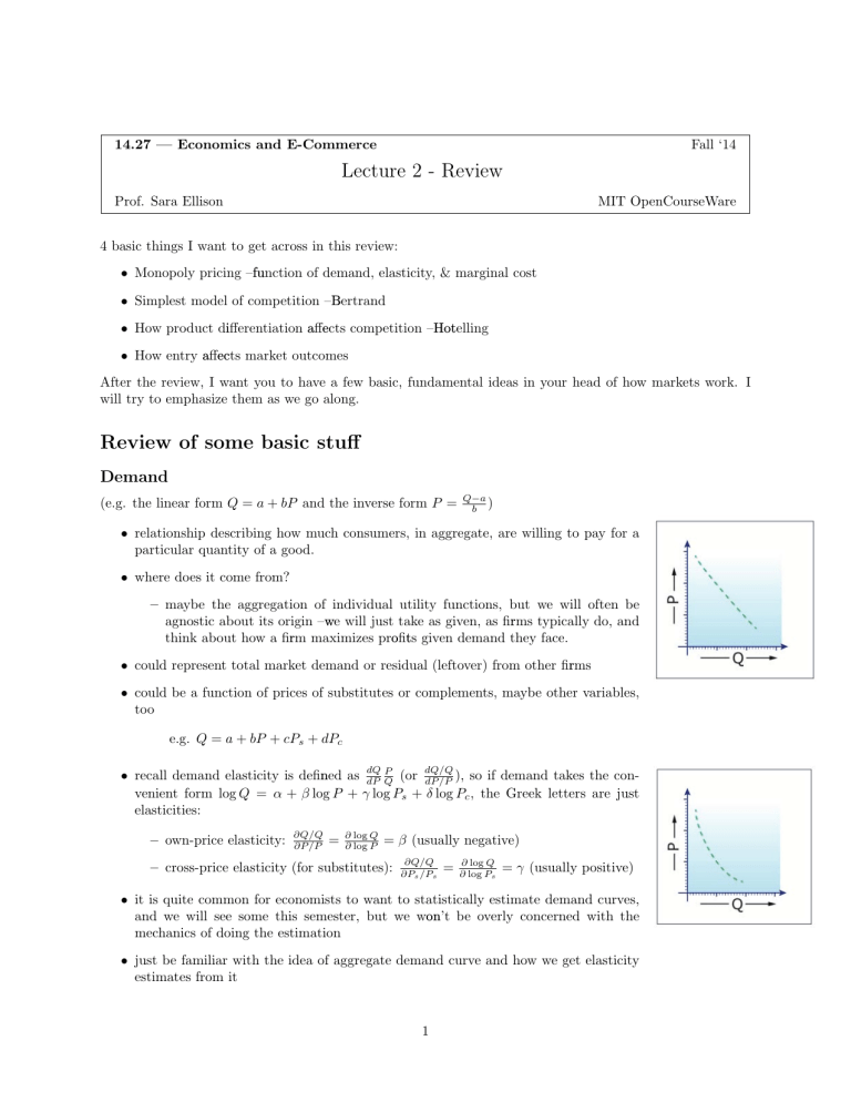
14.27 — Economics and E-Commerce Fall ‘14 ‘ Lecture 2 - Review Prof. Sara Ellison MIT OpenCourseWare 4 basic things I want to get across in this review: • Monopoly pricing –function –fu of demand, elasticity, & marginal cost • Simplest model of competition –B –Bertrand • How product differentiation iff affe –Hot affects competition –Hotelling • How entry affects affec market outcomes After the review, I want you to have a few basic, fundamental ideas in your head of how markets work. I will try to emphasize them as we go along. Review of some basic stuff Demand (e.g. the linear form Q = a + bP and the inverse form P = Q�a b ) • relationship describing how much consumers, in aggregate, are willing to pay for a particular quantity of a good. • where does it come from? – maybe the aggregation of individual utility functions, but we will often be agnostic about its origin –w –we will just take as given, as fir firms typically do, and think about how a fir firm maximizes profits ofit given demand they face. • could represent total market demand or residual (leftover) from other firms fir • could be a function of prices of substitutes or complements, maybe other variables, too e.g. Q = a + bP + cPs + dPc dQ/Q P • recall demand elasticity is defined fin as dQ dP Q (or dP/P ), so if demand takes the con­ venient form log Q = α + β log P + γ log Ps + δ log Pc , the Greek letters are just elasticities: – own­price elasticity: ∂Q/Q ∂P/P = ∂ log Q ∂ log P = β (usually negative) – cross­price elasticity (for substitutes): ∂Q/Q ∂Ps /Ps = ∂ log Q ∂ log Ps = γ (usually positive) • it is quite common for economists to want to statistically estimate demand curves, and we will see some this semester, but we won’t on’ be overly concerned with the mechanics of doing the estimation • just be familiar with the idea of aggregate demand curve and how we get elasticity estimates from it 1 Lecture 2 Review 14.27, Fall ‘14 ‘ Costs • total, marginal, average variable, etc. • just be aware of two types of costs included in the total cost C(Q): – fi fixed costs, F , are independent of output (e.g., building a brewery, setting up a website) – marginal cost, c or c(Q), is the incremental cost of producing one additional unit (e.g., additional fuel needed for extra passenger on an airplane, wholesale cost of goods being resold) • we often assume for modeling purposes that marginal costs are constant (c) fixed or variable depends on the range of production • sometimes whether a cost is fix you’re ou’ considering – e.g., if output fluctuates office space and staff fine, otherwise need to expand or flu ± 20%, current offic aff is fin contract Monopoly behavior • monopolist maximizes profit ofi • has costs C(Q) (where C is total cost, not marginal cost) and faces inverse demand P (Q) • wants to max P (Q)Q � C(Q) for Q, via first­order fir condition: P ' (Q)Q + P (Q) � C ' (Q) = 0 MR MC rewrite: P (Q) � C ' (Q) P (Q) = �QP ' (Q) P (Q) = �1 P ∂Q (where E = ) E Q ∂P Lerner Index, describes markups that firms set over marginal cost 2 Lecture 2 Review 14.27, Fall ‘14 ’r higher when demand is inelastic • so elasticities determine markups & they’re fi • also note that price does not depend on fixed costs, only marginal fi This is a very powerful & important result for our intuition of how firms price. I wrote this down in the monopoly case, but intuition (sometimes) carries over to non-monopoly case if P (Q) is residual demand. Strategic Behavior in Oligopoly Markets ’ been talking about firms So far this semester, we’ve fir making decisions in isolation - monopolists must consider consumers when deciding how to price, how many & what quality products to off offer, etc, but not competition. ’ a useful benchmark and, in fact, some of the results we saw in monopoly have counterpart results with It’s similar fla flavor in markets where multiple fi firms operate. One important element these models did not capture: fi fi affe you, your actions affect affe them, if you’re ’r a firm operating in a market with other firms, their actions affect affe ’ what we’ll e’ all about next and for and all of you should consider those affects when making decisions. That’s most of the remainder of the semester. Bertrand Paradox: developed by Joseph Bertrand in 1883 fi Let’s start with the simplest model of two firms competing in price that we could write down fi fi • assume 2 firms (generalizes in straight-forward way to n firms) • identical products, so consumers buy from producer with lowest price fi • firms set prices and there is a split market if prices are equal, so the monopoly model is nonstrategic • with market aggregate demand is Q = D(P ) and constant & common marginal cost of production, c: Πi (Pi , Pj ) = (Pi − c)Di (Pi , Pj ) ⎧ if Pi < Pj ⎨ D(Pi ) 1 D(P ) if Pi = Pj where Di (Pi , Pj ) = i ⎩ 2 0 if Pi > Pj • fi al’ price) & non cooperatively firms choose prices simultaneously (they cannot observe rival’s The common solution is a concept in game theory known as a Nash equilibrium. For prices, this is a pair (P1∗ , P2∗ ) where each fi firm’s ’s price maximizes its profit ofit given the other fi firms price, so no one wants to deviate from the equilibrium. Formally, this is: Πi (Pi∗ , Pj∗ ) ≥ Πi (Pi , Pj∗ ) What is that equilibrium? P1∗ = P2∗ = c Proof: • suppose P1∗ > P2∗ > c – firm 1 has zero demand & zero profit fi rofi – if, instead, P1 = P2∗ − E, it obtains entire demand D(P2∗ − E) and has positive margin P2∗ − E − c (and therefore positive profit) ofi ⇒⇐ • now suppose P1∗ = P2∗ > c −c) D(P ∗ )(P ∗ − 1 1 – profit rofi of firm fi 1 is but if it reduces price to P1∗ − E, its profit rofi becomes 2 ∗ ∗ D(P1 − E)(P1 − E − c), which is greater for small E ⇒⇐ 3 Lecture 2 Review • now suppose P1∗ > P2∗ 14.27, Fall ‘14 =c – fi firm 2 makes no profit ofit & could raise its price slightly, still supply all demand, and make positive rofi ⇒⇐ profit fir • so both firms price at marginal cost and make no profit ofi Notes: –e • this result suggests the monopoly results we saw before are very special –even a duopoly restores perfect competition • we call it a paradox, though, because it seems so at odds with casual empiricism • we also call it a paradox because we think all fi firms incur fix fixed costs of some type & if they enter even a duopoly market of this type they can never cover their fi fixed costs Discussion The Bertrand Paradox is stylized model, for sure, but not an unreasonable setup –the –t results, though are paradoxical. What is going on? There is a special set of important assumptions underlying the results: • consumers assumed to know both prices • demand has this knife-edge quality • firms only set price once fi • firms can meet all demand immediately fi Note: because we can criticize the model does not mean it’s ’s not valuable. It represents a very real tendency that firms must work hard to escape, and these criticisms of the model do suggest ways in which firms fi fir competing can escape the Bertrand Paradox and charge enough to cover fixed costs and make positive profit. fi rofi So, how do firms escape the Bertrand Paradox? fir • product differentiation ff – products are not identical ∗ e.g., spatial differentials between coffee ffe coffe shops or dry cleaners – firms can take actions to further differentiate their products from rivals fi ff ∗ e.g., various characteristics in cars • consumer search – consumers do not always know prices (or product characteristics) of all products ∗ e.g., shopping for rugs in Turkey – firms can take actions to further obfuscate and make search more difficult fi ffic ∗ e.g., it can be costly to drive to five mattress stores and when you do, retailers ffe fiv different rename particular models of mattress to make comparison across retailers difficult. ffic • repeated interactions – firms don’t fi ’ simply meet once and set price once. it turns out that many more equilibria are possible when firms interact over and over. fi ∗ e.g., gasoline stations across the street from each other 4 Lecture 2 Review 14.27, Fall ‘‘14 • capacity constraints – fi firms who cannot immediately meet all demand are credibly committing not to undercut rivals – fi firms foresee this and may not invest in additional capacity to maintain this commitment ∗ think about two hotels in small town, either one too small to satisfy market demand (at typical prices) alone ∗ they will not engage in cutthroat competition then and also won’t ’t increase capacity in the long run because they expect keen competition in the situation of collective overcapacity 5 MIT OpenCourseWare http://ocw.mit.edu 14.27 Economics and E-Commerce Fall 2014 For information about citing these materials or our Terms of Use, visit: http://ocw.mit.edu/terms.
