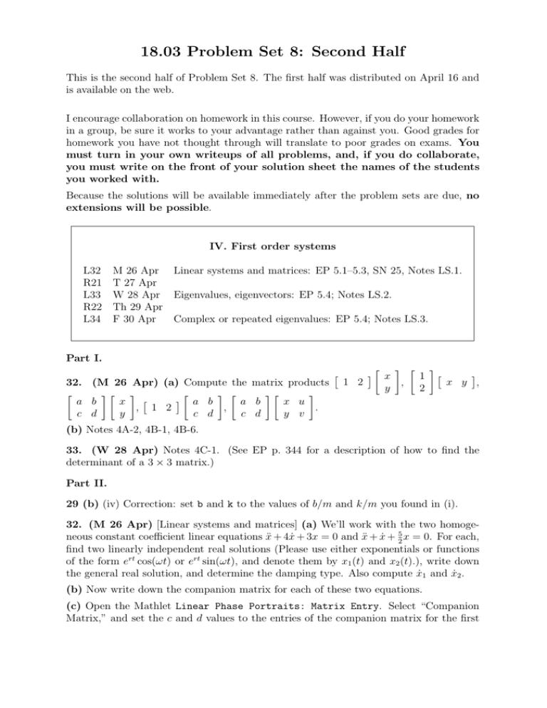
18.03 Problem Set 8: Second Half
This is the second half of Problem Set 8. The first half was distributed on April 16 and
is available on the web.
I encourage collaboration on homework in this course. However, if you do your homework
in a group, be sure it works to your advantage rather than against you. Good grades for
homework you have not thought through will translate to poor grades on exams. You
must turn in your own writeups of all problems, and, if you do collaborate,
you must write on the front of your solution sheet the names of the students
you worked with.
Because the solutions will be available immediately after the problem sets are due, no
extensions will be possible.
IV. First order systems
L32 M 26 Apr Linear systems and matrices: EP 5.1–5.3, SN 25, Notes LS.1.
R21 T 27 Apr
L33 W 28 Apr Eigenvalues, eigenvectors: EP 5.4; Notes LS.2.
R22 Th 29 Apr
L34 F 30 Apr
Complex or repeated eigenvalues: EP 5.4; Notes LS.3.
Part I.
32. (M 26 Apr) (a) Compute the matrix products
�� �
�
� �
��
�
�
�
� a b
x
a b
x u
a b
, 1 2
,
.
y
c d
c d
y v
c d
�
1 2
�
�
� � �
�
x
1 �
x y ,
,
y
2
(b) Notes 4A-2, 4B-1, 4B-6.
33. (W 28 Apr) Notes 4C-1. (See EP p. 344 for a description of how to find the
determinant of a 3 × 3 matrix.)
Part II.
29 (b) (iv) Correction: set b and k to the values of b/m and k/m you found in (i).
32. (M 26 Apr) [Linear systems and matrices] (a) We’ll work with the two homoge­
neous constant coefficient linear equations ẍ + 4ẋ + 3x = 0 and ẍ + ẋ + 52 x = 0. For each,
find two linearly independent real solutions (Please use either exponentials or functions
of the form ert cos(ωt) or ert sin(ωt), and denote them by x1 (t) and x2 (t).), write down
the general real solution, and determine the damping type. Also compute ẋ1 and ẋ2 .
(b) Now write down the companion matrix for each of these two equations.
(c) Open the Mathlet Linear Phase Portraits: Matrix Entry. Select “Companion
Matrix,” and set the c and d values to the entries of the companion matrix for the first
equation. (Note that clicking on a hashmark on a slider sets the value. In some cases
you will have to accept the nearest possible value to the desired value.)
�
�
0 1
For a companion matrix A =
, the colorful window at the upper left shows
c d
(d, −c). You can adjust them by a cursor movement over that plane.
The big window shows the “phase plane” of the system. It displays the trajectories of
a few solutions. Click on the window to produce more. You can clear them all using
[Clear], and return to the original set of trajectories by re-setting one of the c or d
sliders. Do this; return to the originally displayed selection of trajectories.
�
�
x(t)
Since y = ẋ, a solution to u̇ = Au is given by
where x(t) is a solution of
ẋ(t)
ẍ + 4ẋ + 3x = 0 (in this first case). Draw a picture of the phase plane. Each of these
trajectory curves should have an arrow on it indicating the direction of time: please
indicate this on your picture. Identify which of the trajectories correspond to each of the
basic solutions you found in (a). (These will be among the originally chosen trajectories.)
(d) There are some hook-shaped trajectories. The picture doesn’t show a scale; but
suppose that the largest displayed value of x is x = 2. A trajectory crosses the x axis
at x = 1. What is the solution having this as its trajectory assuming that this crossing
occurs at t = 0? Sketch the graph of the corresponding solution x(t) of the original
second order equation.
(e) Write down the general solution having the same trajectory. (Hint: suppose the
solution has x(a) = 1).
(f ) Now set the c and d sliders to the values relevant to the second equation you solved in
(a). Sketch the phase portrait (and include the arrows indicating the direction of time).
Using the same scale as above, what is the solution which passes through (0, 1) at t = 0?
At what other times does this solution cross the y axis? Sketch, roughly, the graphs of
x(t) and of y(t).
(g) In these companion matrix examples, whenever a trajectory crosses the x axis it
seems to do it perpendicularly: its tangent vector is vertical. Explain.
33. (W 28 April) [Eigenvalues, eigenvectors] (a) Find the eigenvalues and eigenvectors
of the companion matrix for ẍ + 4ẋ + 3x = 0. On the x, y plane draw the eigenlines. For
each of the two eigenlines, write down a solution which moves along it. Compare this
with the work you did in 32, especially in part (c).
�
�
2 −4
(b) Find the eigenvalues and eigenvectors of the matrix A =
. Sketch the
1 −3
eigenlines, and for each eigenline write down all the solutions whose trajectories lie on
that line.
(c) Now, invoke Linear Phase Portraits: Matrix Entry again, set a, b, c, and d to
display the phase plane for this matrix, and sketch the phase plane that it displays. Make
sure to include (by clicking on the phase plane) at least one trajectory in each wedge
between eigenlines. Include arrows indicating the direction of time.
MIT OpenCourseWare
http://ocw.mit.edu
18.03 Differential Equations����
Spring 2010
For information about citing these materials or our Terms of Use, visit: http://ocw.mit.edu/terms.