Research Journal of Mathematics and Statistics 5(3): 24-27, 2013
ISSN: 2042-2024, e-ISSN: 2040-7505
© Maxwell Scientific Organization, 2013
Submitted: July 25, 2013
Accepted: August 06, 2013
Published: August 30, 2013
Minimax Estimation of Parameter of Generalized Exponential Distribution
under Square Log Error Loss and MLINEX Loss Functions
Lanping Li
Department of Basic Subjects, Hunan University of Finance and Economics,
Changsha 410205, P.R. China
Abstract: The aim of this paper is to study the minimax estimation of the generalized exponential distribution.
Bayesian estimators and minimax estimators of the parameter of the generalized exponential distribution have been
obtained under the well known weighted square error loss, square log error loss and Modified Linear Exponential
(MLINEX) loss functions. Finally, Monte Carlo simulation is used to compare the efficiency of these minimax
estimators by using mean square error.
Keywords: Bayes estimator, generalized exponential distribution, MLINEX loss, squared log error loss
INTRODUCTION
PRELIMINARIES
Generalized exponential distribution has been used
as an alternative to gamma and Weibull distributions in
many situations by Gupta and Kundu (1999). In recent
years, an impressive array of papers has been devoted
to study the behavioral patterns of the parameters of the
generalized exponential distribution using both classical
and Bayesian approach, a very good summary of this
work can be found in Gupta and Kundu (1999, 2008),
Raqab and Madi (2005) and Singh et al. (2008) and the
references cited there for some recent developments on
GE distribution.
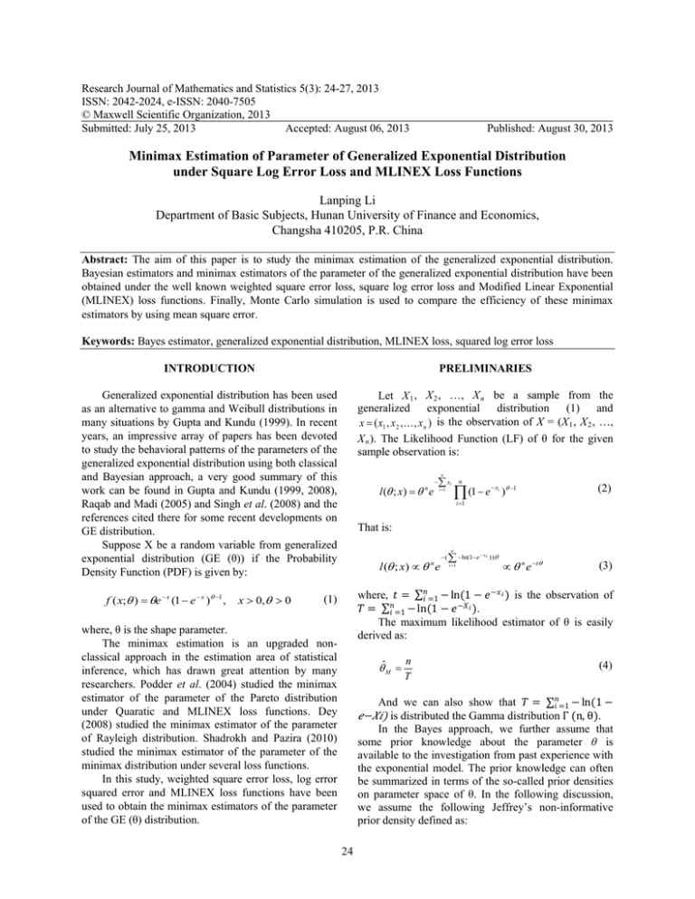
Suppose X be a random variable from generalized
exponential distribution (GE (θ)) if the Probability
Density Function (PDF) is given by:
Let X 1 , X 2 , …, X n be a sample from the
generalized exponential distribution (1) and
x = ( x1 , x 2 ,  , x n ) is the observation of X = (X 1 , X 2 , …,
X n ). The Likelihood Function (LF) of θ for the given
sample observation is:
f ( x;θ ) = θe − x (1 − e − x )θ −1 ,
x > 0,θ > 0
l (θ ; x) = θ e
n
−
n
∑ xi
i =1
n
∏ (1 − e
− xi θ −1
)
(2)
∝ θ n e −t θ
(3)
i =1
That is:
l (θ ; x) ∝ θ e
n
−(
n
∑ −ln(1−e − xi ) )θ
i =1
where, 𝑡𝑡 = ∑𝑛𝑛𝑖𝑖=1 − ln(1 − 𝑒𝑒 −𝑥𝑥 𝑖𝑖 ) is the observation of
𝑇𝑇 = ∑𝑛𝑛𝑖𝑖=1 − ln(1 − 𝑒𝑒 −𝑋𝑋 𝑖𝑖 ).
The maximum likelihood estimator of θ is easily
derived as:
(1)
where, θ is the shape parameter.
The minimax estimation is an upgraded nonclassical approach in the estimation area of statistical
inference, which has drawn great attention by many
researchers. Podder et al. (2004) studied the minimax
estimator of the parameter of the Pareto distribution
under Quaratic and MLINEX loss functions. Dey
(2008) studied the minimax estimator of the parameter
of Rayleigh distribution. Shadrokh and Pazira (2010)
studied the minimax estimator of the parameter of the
minimax distribution under several loss functions.
In this study, weighted square error loss, log error
squared error and MLINEX loss functions have been
used to obtain the minimax estimators of the parameter
of the GE (θ) distribution.
θˆM =
n
T
(4)
And we can also show that 𝑇𝑇 = ∑𝑛𝑛𝑖𝑖=1 − ln(1 −
𝑒𝑒−𝑋𝑋𝑖𝑖) is distributed the Gamma distribution Γ (n, θ).
In the Bayes approach, we further assume that
some prior knowledge about the parameter θ is
available to the investigation from past experience with
the exponential model. The prior knowledge can often
be summarized in terms of the so-called prior densities
on parameter space of θ. In the following discussion,
we assume the following Jeffrey’s non-informative
prior density defined as:
24
Res. J. Math. Stat., 5(3): 24-27, 2013
π (θ ) ∝
1
θ
(5)
, θ >0
h(θ | X ) =
In Bayesian estimation, the loss function plays an
important role and the squared error loss as the most
common symmetric loss function is widely used due to
its great analysis properties. And the weighted Square
Error Loss Function (SELF):
L(θ , δ ) =
(δ − θ )
2
•
•
(11)
Using (10):
Tn ∞
ln θ ⋅ θ n −1e −Tθ dθ
Γ(n) ∫0
d
= ln Γ(n) − ln T =
Ψ (n) − ln T
dr
where,
Ψ ( n)=
d
dn
ln Γ( n)
n−1e
+∞ ln y ⋅ y
= ∫0
Γ( n)
(7)
which is balanced and L(θ , δ ) → ∞ as δ → 0 or ∞ . This
−y
dy
is a Digamma function.
Then the Bayes estimator under the squared log
error loss function is come out to be:
𝛿𝛿
loss is not always convex, it is convex for ≤ 𝑒𝑒 and
𝜃𝜃
concave otherwise, but its risk function has minimum
w.r.t.:
δˆSL = exp[ E (ln θ | X )] =
δˆSL = exp[ E (ln θ | X )]
•
The MLINEX loss function: Varian (1975) and
Zellner (1986) proposed an asymmetric loss function
known as the LINEX function, which is suitable for
situations where overestimation is more costly than
underestimation.
When estimating a parameter θ by 𝜃𝜃� , the MLINEX
is given by (Podder et al., 2004):
 
 − 1 ; ω > 0, c ≠ 0
 
e Ψ (n)
T
(12)
Using (10), the Bayes estimator under the
MLINEX loss function is obtained as:
1  Γ( n − c) 
δˆMML = [ E (θ −c | X )]−1 / c = ⋅ 
T  Γ(n) 
−1 / c
(13)
MINIMAX ESTIMATION
The derivation of minimax estimators depends
primarily on a theorem due to Lehmann which can be
stated as follows:
(8)
Lemma 1: (Lehmann’s Theorem) (Brown, 1968) If
τ = {Fθ ;θ ∈ Θ} be a family of distribution functions and
D a class of estimators of θ. Suppose that δ • ∈ D is a
Bayes estimator against a prior distribution δ • (θ ) on
•
Θ and R (δ • ,θ ) equals constant on Θ ; then δ is a
minimax estimator of θ.
Remark 1: For any prior distribution of θ, under the
MLINEX loss function (8), we can show that the Bayes
estimator of θ, denoted by 𝛿𝛿̂𝑀𝑀𝑀𝑀 , is given by:
δˆML = [ E (θ − c | X )]−1 / c
E[θ −1 | X ] n − 2
=
T
E[θ −2 | X ]
E (ln θ | X )
=
The squared log error loss function: Thus using of
the symmetric loss function may be inappropriate;
Brown (1968) proposed a new loss function for scale
parameter estimation. This loss that is called squared
log error loss is:
 δ c
δ
L(θ , δ ) = ω   − c ln
θ
θ
 
The Bayes estimator under the weighted square
error loss function is given by:
δˆBS =
which is a symmetrical loss function that assigns equal
losses to overestimation and underestimation. However,
in many practical problems, overestimation and
underestimation will make different consequents.
L(θ , δ ) = (ln δ − ln θ ) 2
(10)
This is a Gamma distribution Γ(n, T ) . Then:
(6)
θ2
T n n −1 −Tθ
θ e
Γ( n)
(9)
Bayes estimation: Combining (3) with non-informative
prior (5) using Bayes theorem, the posterior pdf of θ is
given by:
25
Theorem 1: Let X 1 , X 2 , …, X n be a random sample
𝑛𝑛−2
drawn from the density (1), then 𝛿𝛿̂𝐵𝐵𝐵𝐵 =
is the
𝑇𝑇
Res. J. Math. Stat., 5(3): 24-27, 2013
minimax estimator of the parameter θ for the weighted
square error loss (6).
Thus:
E[ln δˆSL ] = E ( Ψ ( n) − ln T )
Theorem 2: Let X 1 , X 2 , …, X n be a random sample
𝑒𝑒 Ψ (𝑛𝑛 )
is the
drawn from the density (1), then 𝛿𝛿̂𝑆𝑆𝑆𝑆 =
ln θ
=
Ψ ( n) − ( Ψ ( n) − ln θ ) =
𝑇𝑇
minimax estimator of the parameter θ for the squared
log error loss (7).
E[ln δˆSL ]2 = E (Ψ (n) − ln T ) 2
=Ψ 2 (n) − 2Ψ (n) E (ln T ) + E[(ln T ) 2 ]
Theorem 3: Let X 1 , X 2 , …, X n be a random sample
drawn from the density (1), then:
1  Γ ( n) 
δˆMML = ⋅ 
T  Γ(n − c) 
1/ c
 Γ ( n) 
K
= , K =

T
 Γ(n − c) 
1/ c
Using the fact:
Proof: First we have to prove the theorem 1. To prove
the theorem we shall use Lehmann’s theorem, which
has been stated before. For this, first we have to find the
Bayes estimator δ of θ. Then if we can show that the
risk of d is constant, then the theorem 1 will be proved.
𝑛𝑛−2
is:
The risk function of the estimator 𝛿𝛿̂𝐵𝐵𝐵𝐵 =
𝑇𝑇
1
Y = Tθ ~ Γ(n,1)
Thus,
Ψ 2 ( n) + =
Ψ ′(n) E[(ln=
Y ) 2 ] E[(ln T + ln θ ) 2 ]
= E[(ln T ) 2 ] + 2 ln θ ⋅ (Ψ (n) − ln θ ) + (ln θ ) 2
Then we get the fact:
E[(ln T ) 2 ] = Ψ 2 (n) + Ψ ′(n) − 2 ln θ ⋅ Ψ (n) + (ln θ ) 2
[(n − 2) E (T ) − 2θ (n − 2) E (T ) + θ ]
−2
2
Then, 𝑅𝑅 (𝜃𝜃) =
−1
2
Therefore E[ln δˆSL ] 2 = Ψ ′( n) + (ln θ ) 2 .
Then R(θ ) = Ψ ′(n) , which is a constant. So,
according to the Lehmann’s theorem it follows that,
𝑒𝑒 Ψ (𝑛𝑛 )
is the minimax estimator for the parameter
𝛿𝛿̂𝑆𝑆𝑆𝑆 =
1
which is a constant. So, according
𝑛𝑛−2
is
to the Lehmann’s theorem it follows that, 𝛿𝛿̂𝐵𝐵𝐵𝐵 =
𝑇𝑇
the minimax estimator for the parameter θ of the
generalized exponential distribution under the quadratic
loss function (7).
Now we are going to prove the theorem 2. The risk
function of the estimator:
δˆSL =
𝑛𝑛−1
𝑇𝑇
θ of the generalized exponential distribution under the
squared log error loss function (8).
Now we give the proof of the case of Theorem 3.
The risk function under the MLINEX loss function (9)
is:
e Ψ (n)
T
 δˆ
R(θ ) = E L θ , δˆMML = wE  MML
 θ

[(
is:
[(
)]
(
)
(
= E[ln δˆSL ] 2 − 2 ln θ ⋅ E ln[δˆSL ] + (ln θ ) 2
n −1
, E (T −2 ) =
)
(
)
But:
(
From the conclusion T ~ Γ(n,θ ) , we have:
θ
)]
c

ˆ

 − c ln δ MML − 1

θ



1

c
= ω  c E δˆMML
− cE ln δˆMML + c ln θ − 1
θ


2
R(θ ) = E L θ , δˆSL = E  ln δˆSL − ln θ 


E (T −1 ) =
2 n −1 − y
∞ (ln y ) y
e
(ln y ) 2 y n −1e − y
Ψ (n)dy
dy − ∫
0
Γ ( n)
Γ ( n)
where, Y ~ Γ(n,1) . Then we can show that:
 (n − 2) / T − θ  2 
  n − 2 
R(θ ) = E  Lθ ,
 
 = E 
θ
T 
 
 

θ2
∞
0
= E[(ln Y ) 2 ] − Ψ 2 (n)
is the minimax estimator of the parameter θ for the
MLINEX loss (8).
=
∫
=
Ψ ′(n)
)
c
= E ( K / T ) c = K c ⋅ E (T −c ) = K c
E δˆMML
θ2
(
(n − 1)(n − 2)
)
Γ(n − c) c
θ =θc
Γ ( n)
K
) ln K − E (ln T )
E ln δˆMML
= E (ln =
T
= ln K + ln θ − Ψ (n)
E (ln T ) = Ψ (n) − ln θ
26
Res. J. Math. Stat., 5(3): 24-27, 2013
Table 1: Estimated value and corresponding ER (𝜃𝜃� )
n
Criteria
𝛿𝛿̂𝑀𝑀𝑀𝑀
10
Estimated value
1.1158
0.1701
ER (𝜃𝜃� )
20
Estimated value
1.0522
0.0638
ER (𝜃𝜃� )
50
Estimated value
1.0221
0.0222
ER (𝜃𝜃� )
75
Estimated value
1.0153
0.0142
ER (𝜃𝜃� )
100
Estimated value
1.0103
0.0104
ER (𝜃𝜃� )
𝛿𝛿̂𝐵𝐵𝐵𝐵
0.8927
0.1118
0.9469
0.0523
0.9812
0.0203
0.9882
0.0133
0.9901
0.0100
𝛿𝛿̂𝑆𝑆𝑆𝑆
1.0605
0.1452
1.0260
0.0587
1.0119
0.0214
1.0086
0.0138
1.0052
0.0102
Then R(θ ) = w[ln K − c + cΨ (n)] , which is a constant.
So, according to the Lehmann’s theorem it follows that,
1
Γ(𝑛𝑛) 1/𝑐𝑐
𝛿𝛿̂𝑀𝑀𝑀𝑀𝑀𝑀 = ∙ [
] is the minimax estimator for the
𝑇𝑇
REFERENCES
Brown, L.D., 1968. Inadmissibility of the usual
estimators of scale parameters in problems with
unknown location and scale parameters. Ann.
Math. Stat., 39: 29-48.
Dey, S., 2008. Minimax estimation of the parameter of
the rayleigh distribution under quadratic loss
function. Data Sci. J., 7: 23-30.
Gupta, R.D. and D. Kundu, 1999. Generalized
exponential distribution. Aust. NZ J. Stat., 41(2):
173-188.
Gupta, R.D. and D. Kundu, 2008. Generalized
exponential distribution: Bayesian estimations.
Comput. Stat. Data Anal., 4: 1873-1883.
Podder, C.K., M.K. Roy, K.J. Bhuiyan and A. Karim,
2004. Minimax estimation of the parameter of the
Pareto distribution for quadratic and MLINEX loss
functions. Pak. J. Stat., 20(1): 137-149.
Raqab, M.Z. and T. Madi, 2005. Bayesian inference for
the generalized exponential distribution. J. Stat.
Comput. Sim., 75(10): 841-852.
Shadrokh, A. and H. Pazira, 2010. Minimax estimation
on the minimax distribution. Int. J. Stat. Syst., 5(2):
99-118.
Singh, R., S.K. Singh, V. Singh and G.P. Singh, 2008.
Bayes estimator of generalized exponential
parameters under linex loss function using
Lindley’s approximation. Data Sci. J., 7: 65-75.
Varian, H.R., 1975. A Bayesian Approach to Real
Estate Assessment. In: Fienberg, S.E. and
A. Zellner (Eds.), Studies in Bayesian
Econometrics and Statistics in Honor of Leonard
J. Savage. North Holland Publishing Co.,
Amsterdam, pp: 195-208.
Zellner, A., 1986. Bayesian estimation and prediction
using asymmetric loss functions. J. Am. Stat.
Assoc., 81: 446-451.
The risks under squared-error loss of the estimates
are considered to compare the different estimators of
the parameter θ of the generalized exponential
distribution that are obtained by maximum likelihood
and minimax methods for weighted square error loss,
squared log error error loss and MLINEX loss
functions:
•
Based on the given value θ = 1.0, a sample of size
n is then generated from the density of the
Generalized Exponential distribution (1), which is
considered to be the informative sample
The MLE and minimax estimators is calculated
based on Section 3 and in loss function (6),
c = -1.0, 1.0, 2.0
Steps (1) to (2) are repeated N = 5000, times and
the risks under squared error loss of the estimates
are computed by using:
1
ER(θˆ) =
N
N
∑ (θˆ − θ )
𝛿𝛿̂𝑀𝑀𝑀𝑀𝑀𝑀 c = 2.0
0.9468
0.1156
0.9729
0.0529
0.9914
0.0205
0.9950
0.0134
0.9951
0.0100
This study is partially supported by Foundation of
Hunan Educational Committee, No. 12C0563.
Γ(𝑛𝑛−𝑐𝑐)
EMPIRICAL STUDY
•
𝛿𝛿̂𝑀𝑀𝑀𝑀𝑀𝑀 c = 1.0
1.0042
0.1269
0.9995
0.0551
1.0017
0.0208
1.0018
0.0136
1.0002
0.0101
ACKNOWLEDGMENT
parameter θ of the generalized exponential distribution
under the MLINEX loss function (9).
•
𝛿𝛿̂𝑀𝑀𝑀𝑀𝑀𝑀 c = -1.0
1.1158
0.1701
1.0522
0.0638
1.0221
0.0222
1.0153
0.0142
1.0103
0.0104
2
i =1
where 𝜃𝜃�𝑖𝑖 is the estimate at the ith run.
CONCLUSION
The estimated values of the parameter and ER of
the estimators are computed by the Monte-Carlo
Simulation method from the generalized exponential
distribution (1) with θ = 1.0 . It is seen that for small
sample sizes (n<50), minimax estimators for MLINEX
loss function when c = 1.0 appear to be better than the
other minimax estimators. But for large sample sizes
(n>50), all the three estimators have approximately the
same ER. The obtained results are demonstrated in the
Table 1.
27