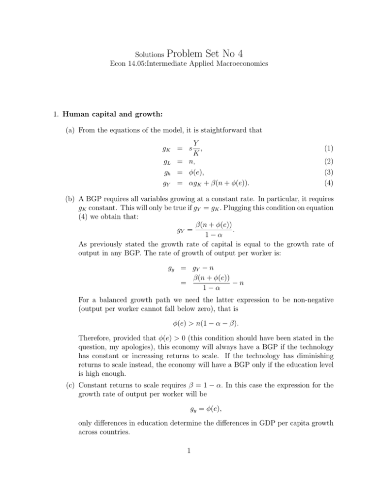
Solutions Problem Set No 4
Econ 14.05:Intermediate Applied Macroeconomics
1. Human capital and growth:
(a) From the equations of the model, it is staightforward that
Y
,
K
= n,
= φ(e),
= αgK + β(n + φ(e)).
gK = s
(1)
gL
gh
gY
(2)
(3)
(4)
(b) A BGP requires all variables growing at a constant rate. In particular, it requires
gK constant. This will only be true if gY = gK . Plugging this condition on equation
(4) we obtain that:
β(n + φ(e))
gY =
.
1−α
As previously stated the growth rate of capital is equal to the growth rate of
output in any BGP. The rate of growth of output per worker is:
gy = gY − n
β(n + φ(e))
=
−n
1−α
For a balanced growth path we need the latter expression to be non-negative
(output per worker cannot fall below zero), that is
φ(e) > n(1 − α − β).
Therefore, provided that φ(e) > 0 (this condition should have been stated in the
question, my apologies), this economy will always have a BGP if the technology
has constant or increasing returns to scale. If the technology has diminishing
returns to scale instead, the economy will have a BGP only if the education level
is high enough.
(c) Constant returns to scale requires β = 1 − α. In this case the expression for the
growth rate of output per worker will be
gy = φ(e),
only differences in education determine the differences in GDP per capita growth
across countries.
1
(d) Under
From this
output
study, time
this reduces
rate of
level of
immediately
in e should
long run.
2. The role of
(a) The new
implies
capital
standard
k
Figure 1:
2
·
(b) Now we have k(t) = sB(1 − τ )k α − (n + δ)k = sτ β k αβ (1 − τ )k α − (n + δ)k =
sτ β (1 − τ )k α(1+β) − (n + δ)k. That implies that the growth rate is gk = sτ β (1 −
τ )k α(1+β)−1 − (n + δ). Consequently, what happens in the long run depends on
wether α(1 + β) � 1, or which is the same, β � 1−α
. If β > 1−α
then α(1 + β) > 1,
α
α
which implies that as we accumulate capital, marginal product increases every
time more and more. So we have increasing marginal product. The growth rate
then α(1 + β) < 1, which
increases forever and the economy explodes. If β < 1−α
α
implies that although marginal product is not as decreasing as before, it still is
decreasing. As we know, this implies the economy converges to a long run level of
capital per effective labor because this is nothing more than the standard Solow
. In that case gk = sτ β (1−τ )−(n+δ),
model. The interesting case is when β = 1−α
α
which implies we have a constant growth rate for the level of capital per effective
worker. We have endogenous growth!
, gk = sτ β (1 − τ ) − (n + δ). If we maximize this with
(c) In the case with β = 1−α
α
respect to τ, the F.O.C. is
sβτ β−1 (1 − τ ) − sτ β = 0 ⇔ βτ −1 (1 − τ ) = 1 ⇔
β
.
τ∗ =
1+β
Why is there a τ that maximizes growth? τ has two effects. It takes resources
away from the private economy, which reduces growth. But the government uses
the taxes for producing goods, say roads, that create an externality to private
production, and this increases growth. The higher is β, the more productive is
the government relative to the private sector, and the bigger should be the tax.
·
(d) In that case we know k(t) = s(1 − τ )k α − (n + δ)k. This means that we only have
the negative effect of taxation as the government is stealing the taxes. In that case
endogenous growth does not arise because there are no externalities and we have
a lower capital than without government. This model helps understanding how
different governments affect the long run properties of a economy. In countries
with corrupt governments, the economy will stagnate, while in countries with
productive governments, high growth rates can be sustained.
3. Appropriate technology and the role of education
(a) If we take logs in the expression for the growth rate of technology we get log gA =
log A − log A∗ + log g ∗ . Differentiating with respect to time we get
·
·
· ∗
gA
A A
= − ∗ = gA − gA∗ .
gA
A A
And using the expression for gA we get
·
A
gA
A
= ∗ g ∗ − g ∗ = ( ∗ − 1)g ∗ ,
gA
A
A
3
which is negative as we assumed A < A∗ . So the country starts with a lower growth
rate, and the growth rate decreases over time. This means that the distance of
the country to the world technology increases over time, technologies diverge.
This tell us that if you need certain amount of technology to understand new
technologies, poor countries with backward initial technologies not only won’t
catch up with the rest of the world, but they will diverge for ever.
(b) Now the
backward country starts with a bigger growth rate as A < A∗ and
.
gA =
A(t)
A(t)
=
A(t)∗ ∗
g .
A(t)
Following the same steps as before we get:
·
A(t)∗ ∗
gA
A(t)∗ ∗
g = (1 −
)g
= gA∗ − gA = g ∗ −
gA
A(t)
A(t)
which is negative and goes to 0 as A approaches A∗ . So the backward country
starts with a higher growth rate than the world, and the growth rate decreases as
this country gets closer to the growth frontier. This keeps going until it catches
up. So in that case we have convergence in the growth rates and the levels of
technology.
(c) The expression for the growth rate of the growth rate is now
·
A(t)∗ ∗
gA
A(t)∗ ∗
∗
∗
= gA − gA + e = g −
g + e = (1 −
)g e
gA
A(t)
A(t)
which can be positive now. So, among backward countries, those with high levels
of human capital growth may catch up with the world, while those with little
growth in human capital will diverge forever.
(d) We already discussed all the mechanisms. Both mechanisms might be relevant in
the real world. It is quite intuitive that some technologies are not appropriate for
the poor countries because they are developed in the rich countries, and the poor
lack the human capital, and their technology is too backward to fully benefit of
these new technologies. But it also makes sense to think that, the more backward
a country is, the more it can benefit from innovations. We could recommend a
backward country to accumulate human capital by putting in place an appropriate
education system and making sure it is actually used.
4