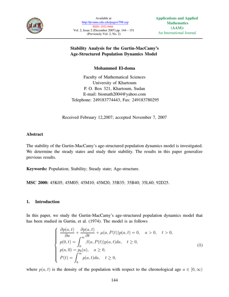
Available at
http://pvamu.edu.edu/pages/398.asp
ISSN: 1932-9466
Vol. 2, Issue 2 (December 2007) pp. 144 – 151
(Previously Vol. 2, No. 2)
Applications and Applied
Mathematics
(AAM):
An International Journal
Stability Analysis for the Gurtin-MacCamy’s
Age-Structured Population Dynamics Model
Mohammed El-doma
Faculty of Mathematical Sciences
University of Khartoum
P. O. Box 321, Khartoum, Sudan
E-mail: biomath2004@yahoo.com
Telephone: 249183774443, Fax: 249183780295
Received February 12,2007; accepted November 7, 2007
Abstract
The stability of the Gurtin-MacCamy’s age-structured population dynamics model is investigated.
We determine the steady states and study their stability. The results in this paper generalize
previous results.
Keywords: Population; Stability; Steady state; Age-structure.
MSC 2000: 45K05; 45M05; 45M10; 45M20; 35B35; 35B40; 35L60; 92D25.
1.
Introduction
In this paper, we study the Gurtin-MacCamy’s age-structured population dynamics model that
has been studied in Gurtin, et al. (1974). The model is as follows

∂p(a, t) ∂p(a, t)


+
+ µ(a, P (t))p(a, t) = 0, a > 0, t > 0,


∂a
Z ∞ ∂t



 p(0, t) =
β(a, P (t))p(a, t)da, t ≥ 0,
(1)
0


p(a,
0)
=
p
(a),
a
≥
0,

Z ∞0




 P (t) =
p(a, t)da, t ≥ 0,
0
where p(a, t) is the density of the population with respect to the chronological age a ∈ [0, ∞)
144
AAM: Intern. J., Vol. 2, Issue 2 (December 2007), [Previously Vol. 2, No. 2]
at time t ≥ 0; P (t) =
Z
145
∞
p(a, t)da is the total population size at time t; β(a, P (t)), µ(a, P (t))
0
are, respectively, the birth rate i.e. the average number of offspring, per unit time, produced by
an individual of age a when the population size is P (t), and the mortality
Z rate i.e. the death rate
∞
at age a, per unit population, when the population size is P (t); p(0, t) =
is the number of births, per unit time, when the population size is P (t).
β(a, P (t))p(a, t)da
0
We study problem (1) under the following general assumptions:

0 ≤ p0 (a) ∈ L1 (R+ ), R+ = [0, ∞);



β(a, P (t)) > 0, µ(a, P (t)) > 0, µ(a, P (t)) ∈ C(R+ × R+ );
β (a, P ), µP (a, P ) exist for ∀a ≥ 0, P ≥ 0;


 P
β(., P ), βP (., P ), µ(., P ), µP (., P ) ∈ C(R+: L∞ (R+ )).
(2)
In Gurtin, et al. (1974) problem (1) is described and existence and uniqueness results via a fixed
point theorem are obtained as well as the local asymptotic stability of a nontrivial steady state
when all the roots of the corresponding characteristic equation have negative real parts. Since
then several authors have attempted to study the stability of special cases of this model in order
to determine conditions under which all the roots of the corresponding characteristic equation
have negative real parts, for example, see Weinstock, et al. (1987), Di Blasio, et al. (1982), and
Iannelli(1995) and the references therein. Some recent results involving the global stability and
global boundedness of solution are given in Ianneli(1995), Iannelli, et al. (2002), Bekkal-Brikci,
el al. (2007), and El-Doma (Preprint to appear).
In this paper, we study problem (1) and determine its steady states and examine their stability.
We show that if R(0) < 1, see section 2 for the definition of R(P ), then the trivial steady state
is locally asymptotically stable, and if R(0) > 1, then the trivial steady state is unstable. We also
determine sufficient conditions for the local asymptotic stability of a nontrivial steady state P∞ ,
and show that if R0 (P∞ ) > 0, then a nontrivial steady state is unstable.
The organization of this paper as follows: in section 2 we determine the steady states; in section
3 we study the stability of the steady states; in section 4 we conclude our results.
2.
The Steady States
In this section, we determine the steady states of problem (1). A steady state of problem (1)
satisfies the following:

dp∞ (a)


+ µ(a, P∞ )p∞ (a) = 0, a > 0,


da


Z ∞

(3)
p∞ (0) =
β(a, P∞ )p∞ (a)da,

0

Z

∞



 P∞ =
p∞ (a)da.
0
From (3), by solving the differential equation, we obtain that
p∞ (a) = p∞ (0)π(a, P∞ ),
(4)
146
Mohammed El-doma
where π(a, P∞ ) is defined as
π(a, P ) = e−
Ra
0
µ(τ,P )dτ
,
is the probability of survival to age a when the population size is P. Also, from (3) and (4), we
obtain that p∞ (0) satisfies the following:
Z ∞
p∞ (0) = p∞ (0)
β(a, P∞)π(a, P∞ )da.
(5)
0
Accordingly, from (5), we conclude that either p∞ (0) = 0 or P∞ satisfies the following:
Z ∞
1=
β(a, P∞ )π(a, P∞ )da.
(6)
0
In order to facilitate our writing, we define a threshold parameter R(P ) by
Z ∞
R(P ) =
β(a, P )π(a, P )da,
(7)
0
which is interpreted as the number of children expected to be born to an individual, in a life
time, when the population size is P.
We note that from equation (4), p∞ (0) = Z
P∞
∞
, and accordingly, either p∞ (a) ≡ 0
π(a, P∞ )da
0
or p∞ (a) is completely determined by a solution P∞ of equation (6).
In the following theorem, we describe the steady states of problem (1), the proof of the theorem
is straightforward and therefore, is omitted.
Theorem 2.1:
(a) Problem (1) has the trivial steady state, P∞ = 0, as a steady state.
(b) All nontrivial solutions of, R(P∞ ) = 1, are nontrivial steady states of problem (1).
3.
Stability of the Steady States
In this section, we study the stability of the steady states for problem (1) as given by Theorem
2.1.
To study the stability of a steady state p∞ (a), which is a solution of (3) and is given by equation
(4), we linearize problem (1) at p∞ (a) in order to obtain a characteristic equation, which in turn
will determine conditions for the stability. To that end, we consider a perturbation ω(a, t) defined
by ω(a, t) = p(a, t) − p∞ (a), where p(a, t) is a solution of problem (1). Accordingly, we obtain
that ω(a, t) satisfies the following:

∂ω(a, t) ∂ω(a, t)


+
+ µ(a, P∞ )ω(a, t) + p∞ (a)µP (a, P∞ )W (t) = 0, a > 0, t > 0,


∂a
Z ∞ ∂t
Z ∞



 ω(0, t) =
β(a, P∞ )ω(a, t)da + W (t)
βP (a, P∞ )p∞ (a)da, t ≥ 0,
(8)
0
0


ω(a,
0)
=
p
(a)
−
p
(a),
a
≥
0,
0
∞

Z ∞




 W (t) =
ω(a, t)da, t ≥ 0.
0
AAM: Intern. J., Vol. 2, Issue 2 (December 2007), [Previously Vol. 2, No. 2]
147
By substituting ω(a, t) = f(a)eλt in (8), where λ is a complex number, and straightforward
calculations, we obtain the following characteristic equation:
1=
Z
Z
∞
e−λaβ(a, P∞ )π(a, P∞ )da +
0
Z
∞
Z
a
∞
e−λa π(a, P∞)da
0
e−λ(a−σ) p∞ (a)µP (σ, P∞ )dσda
0
0
Z ∞Z a
hZ ∞
i
−λ(a−σ)
×
βP (a, P∞ )p∞ (a)da −
e
β(a, P∞)p∞ (a)µP (σ, P∞ )dσda .
1+
0
0
(9)
0
In the following theorem, we describe the stability of the trivial steady state p∞ (a) ≡ 0.
Theorem 3.1: The trivial steady state p∞ (a) ≡ 0, is locally asymptotically stable if R(0) < 1,
and is unstable if R(0) > 1.
Proof: We note that for the trivial steady state p∞ (a) ≡ 0, P∞ = 0, and therefore, from the
characteristic equation (9), we obtain the following characteristic equation:
1=
Z
∞
e−λa β(a, 0)π(a, 0)da.
(10)
0
To prove the local asymptotic stability of the trivial steady state, we note that if R(0) < 1, then
equation (10) can not be satisfied for any λ with Reλ ≥ 0 since
Z
∞
β(a, 0)π(a, 0)e
−λa
0
Z
da ≤
∞
β(a, 0)π(a, 0)e−aReλda,
0
≤ R(0) < 1.
Accordingly, the trivial steady state is locally asymptotically stable if R(0) < 1.
To prove the instability of the trivial steady state when R(0) > 1, we note that if we define a
function g(λ) by
g(λ) =
Z
∞
β(a, 0)π(a, 0)e−λada,
0
and suppose that λ is real, then we can easily see that g(λ) is a decreasing function if λ > 0,
g(λ) −→ 0 as λ −→ +∞, and g(0) = R(0). Therefore, if R(0) > 1, then there exists λ∗ > 0
such that g(λ∗ ) = 1, and hence the trivial steady state is unstable. This completes the proof of
the theorem.
In the next theorem, we give a condition for the instability of a nontrivial steady state.
Theorem 3.2: A nontrivial steady state is unstable if R0 (P∞ ) > 0.
148
Mohammed El-doma
Proof: We note that the characteristic equation (9) can be rewritten as
Z ∞
1 =
e−λa β(a, P∞)π(a, P∞ )da
Z ∞
Z0 ∞ Z a
−λ(a−σ)
−λa
+
e
p∞ (a)µP (σ, P∞ )dσda
e β(a, P∞)π(a, P∞ )da − 1
0
0
0
Z ∞
+
e−λa π(a, P∞)da ×
(11)
0Z
Z ∞Z a
∞
−λ(a−σ)
βP (a, P∞ )p∞ (a)da −
e
β(a, P∞)p∞ (a)µP (σ, P∞ )dσda
0
0
0
:= G(λ).
Now, suppose that R0 (P∞ ) > 0, then from the characteristic equation (11), we obtain that G(0) =
1 + R0 (P∞ )P∞ > 1, and G(λ) −→ 0 as λ −→ +∞. Accordingly, ∃λ∗ > 0 such that G(λ∗ ) = 1,
and hence a nontrivial steady state is unstable. This completes the proof of the theorem.
In the next theorem, we prove that, λ = 0, is a root of the characteristic equation (11) iff
R0 (P∞ ) = 0.
Theorem 3.3: λ = 0 is a root of the characteristic equation (11) iff R0 (P∞ ) = 0.
Proof: We note that if λ = 0, then using equation (6), the characteristic equation (11) becomes
R0 (P∞ ) = 0. This completes the proof of the theorem.
To obtain further stability results, we note that by suitable changes of the variables of the
integrations, we can rewrite the characteristic equation (11) in the following form:
Z ∞
Z ∞
−λa
1 =
e
β(a, P∞)π(a, P∞ ) −
p∞ (σ)µP (σ − a, P∞ )dσ
0
a
Z ∞
+ π(a, P∞ )
βP (b, P∞ )p∞ (b)db
(12)
0
Z aZ ∞
+
p∞ (b)π(σ, P∞)µP (σ + b − a, P∞ ) [β(b, P∞ ) − β(σ, P∞)] dσdb da.
0
a−b
In the next theorem, we give our first sufficient condition for the local asymptotic stability of a
nontrivial steady state. We note that contrary to our results in this paper, most stability results are
obtained for special cases of problem (1), for example, see Weinstock, et al. (1987), Di Blasio,
et al. (1982), and Iannelli(1995) and the references therein.
Theorem 3.4: Suppose that the following hold:
Z ∞
1. φ(a, P∞ ) = β(a, P∞)π(a, P∞ ) −
p∞ (σ)µP (σ − a, P∞ )dσ
a
Z ∞
+ π(a, P∞)
βP (b, P∞ )p∞ (b)db
(13)
Z aZ ∞ 0
+
p∞ (b)π(σ, P∞)µP (σ + b − a, P∞ ) [β(b, P∞ ) − β(σ, P∞ )] dσdb ≥ 0,
0
a−b
∀ a ≥ 0,
AAM: Intern. J., Vol. 2, Issue 2 (December 2007), [Previously Vol. 2, No. 2]
149
2. R0 (P∞ ) < 0.
Then a nontrivial steady state is locally asymptotically stable.
Proof: We note that from the characteristic equation (12), we obtain that
Z ∞
1=
e−λa φ(a, P∞ )da.
(14)
0
And therefore, if we assume that Reλ ≥ 0, then from equation (14), we obtain
Z ∞
Z ∞
−λa
e−aReλφ(a, P∞ )da
e φ(a, P∞ )da ≤
0
Z0 ∞
≤
φ(a, P∞ )da
0
= 1 + R0 (P∞ )P∞
< 1.
Accordingly, the characteristic equation (12) is not satisfied for any λ with real Reλ ≥ 0, and
hence a nontrivial steady state is locally asymptotically stable. This completes the proof of the
theorem.
In the next result, we give a corollary to Theorem 3.4, and the proof of this corollary is
straightforward, and therefore, is omitted.
Corollary 3.5: Suppose that the following hold:
1) β(a, P ) = β(P ), ∀a ≥ 0,
h
i Z
0
2) π(a, P∞ ) β(P∞ ) + β (P∞ )P∞ −
3) R0 (P∞ ) < 0.
∞
p∞ (σ)µP (σ − a, P∞ )dσ ≥ 0, ∀a ≥ 0,
a
Then a nontrivial steady state is locally asymptotically stable.
In the next theorem, we give our second sufficient condition for the local asymptotic stability of
a nontrivial steady state.
Z ∞
Theorem 3.6: Suppose that
φ(a, P∞ )da < 1, where φ is given by equation (13). Then a
0
nontrivial steady state is locally asymptotically stable.
Proof: Suppose that Reλ ≥ 0, then from the characteristic equation (12), we obtain
Z ∞
Z ∞
−λa
1=
e φ(a, P∞ )da ≤
e−aReλ φ(a, P∞ )da
0
Z0 ∞ ≤
φ(a, P∞ )da
0
< 1.
Accordingly, the characteristic equation (12) is not satisfied for any λ with real Reλ ≥ 0, and
hence a nontrivial steady state is locally asymptotically stable. This completes the proof of the
theorem.
150
Mohammed El-doma
We note that a similar corollary to corollary 3.5 holds in the case when β is a function of P
only.
Example: If we consider the example given in Gurtin, et al. (1974), where µ(a, P ) = µ(P ); β(a, P ) =
β(P )
β(P )e−αa, α ≥ 0. Then R(P ) =
. And therefore, R0 (P∞ ) < 0, is equivalent to
µ(P ) + α
β 0(P∞ ) < µ0 (P∞ ). And in this case Theorem 3.4 gives the following conditions for the local
asymptotic stability:
0
µ0 (P∞ ) −αa
−β(P∞ )a
−µ(P∞ )a β (P∞ )
1) β(P∞ )e
+ p∞ (0)e
−
e
≥ 0,
β(P∞ )
µ(P∞ )
2) β 0(P∞ ) < µ0 (P∞ ).
Also by Theorem 3.6 and if we assume the positivity condition:
0
µ0 (P∞ ) −αa
−β(P∞ )a
−µ(P∞ )a β (P∞ )
−
e
≥ 0,
β(P∞ )e
+ p∞ (0)e
β(P∞ )
µ(P∞ )
then we obtain the following condition for the local asymptotic stability:
1+
p∞ (0)
[β 0(P∞ ) − µ0 (P∞ )] < 1,
β(P∞ )µ(P∞ )
which clearly satisfies the condition of the theorem when β 0(P∞ ) − µ0 (P∞ ) < 0, which is exactly
the condition R0 (P∞ ) < 0.
4.
Conclusion
In this paper, we studied the stability of the well-known Gurtin-MacCamy’s age-structured
population dynamics model given in their paper Gurtin, et al.(1974). In our results, we obtained
stability results for their general model, however, the stability of special cases of this model has
been given in several papers and books, for example, see Weinstock, et al.(1987), Di Blasio, et al.
(1982), and Iannelli(1995), and the references therein. Some recent results involving the global
stability as well as the global boundedness of solution are given in Iannelli(1995), Iannelli, et al.
(2002), Bekkal-Brikci, el al.(2007), and El-Doma (Preprint to appear).
We determined the steady states of the model and examined their stability. We proved that the
trivial steady state is always a steady state and that there are as many nontrivial steady states as
the solutions of the equation, R(P∞ ) = 1, where R(P ) is the number of children expected to
be born to an individual, over a life time, when the population size is P. Then we studied the
stability of the trivial steady state and showed that if R(0) < 1, then the trivial steady state is
locally asymptotically stable, and if R(0) > 1, then the trivial steady state is unstable.
Furthermore, we studied the stability of a nontrivial steady state and we gave several sufficient
conditions for their local asymptotic stability. We also showed that if R0 (P∞ ) > 0, then a
nontrivial steady state is unstable.
References
AAM: Intern. J., Vol. 2, Issue 2 (December 2007), [Previously Vol. 2, No. 2]
151
Bekkal-Brikci, F., K. Boushaba and O. Arino. Nonlinear age structured model with cannibalism.
Discrete and Continuous Dynamical Systems-Series B. Vol. 7, pp. 201-218, (2007).
Di Blasio, G., M. Iannelli and E. Sinestrari. Approach to Equilibrium in Age Structured Populations with an Increasing Recruitment Process. J. Math. Biol.Vol. 13, pp.371-382, (1982).
El-Doma, M. Age-structured Population Model with Cannibalism. Preprint to appear.
Gurtin, M. E., and R. C. MacCamy. Non-linear age-dependent Population Dynamics. Arch.
Rational Mech. Anal. Vol. 54, pp. 281-300, (1974).
Iannelli, M., M.-Y. Kim E.-J. Park and A. Pugliese. Global boundedness of the solutions to a
Gurtin-MacCamy system. Nonlinear differ. equ. appl. Vol. 9, pp. 197-216, (2002).
Iannelli, M. Mathematical theory of age-structured population dynamics.
Applied mathematics monographs. Vol. 7, CNR., Giardini-Pisa, (1995).
Weinstock, E., C. Rorres. Local stability of an Age-structured Population with density-dependent
fertility and mortality. SIAM J. APPL. MATH. Vol. 47, pp. 589-604, (1987).