Maple Command list
Spring 2011
Helpful commands for Math 2250, 2280. Suggest more and I will add them to this list!
If you see a command "foo" that you like, try it! If you want more information or extra options for foo,
type ?foo in a math field and hit enter...the "foo" help window should open. (You can also find out
about "foo" from the help directory, at the upper right of your Maple window.)
Constants
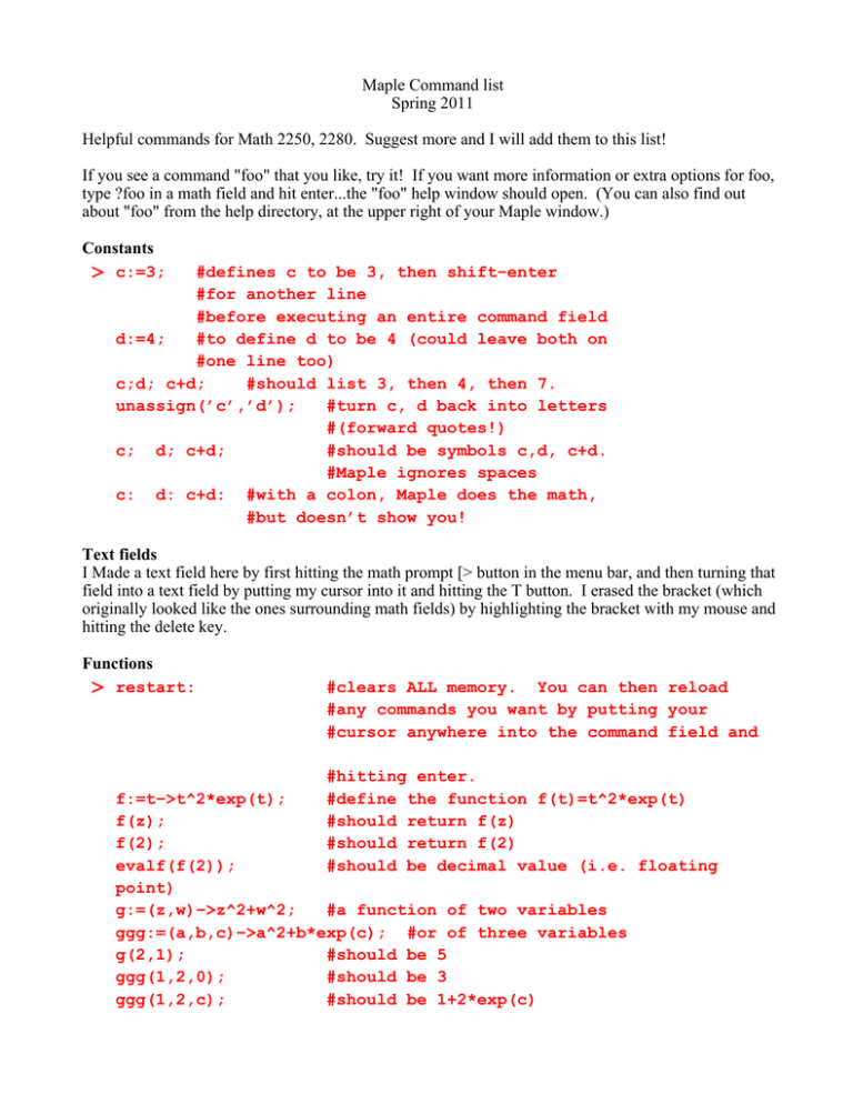
c:=3;
#defines c to be 3, then shift−enter
#for another line
#before executing an entire command field
d:=4;
#to define d to be 4 (could leave both on
#one line too)
c;d; c+d;
#should list 3, then 4, then 7.
unassign(’c’,’d’);
#turn c, d back into letters
#(forward quotes!)
c; d; c+d;
#should be symbols c,d, c+d.
#Maple ignores spaces
c: d: c+d: #with a colon, Maple does the math,
#but doesn’t show you!
Text fields
I Made a text field here by first hitting the math prompt [> button in the menu bar, and then turning that
field into a text field by putting my cursor into it and hitting the T button. I erased the bracket (which
originally looked like the ones surrounding math fields) by highlighting the bracket with my mouse and
hitting the delete key.
Functions
restart:
#clears ALL memory. You can then reload
#any commands you want by putting your
#cursor anywhere into the command field and
#hitting enter.
#define the function f(t)=t^2*exp(t)
#should return f(z)
#should return f(2)
#should be decimal value (i.e. floating
f:=t−>t^2*exp(t);
f(z);
f(2);
evalf(f(2));
point)
g:=(z,w)−>z^2+w^2;
#a function of two variables
ggg:=(a,b,c)−>a^2+b*exp(c); #or of three variables
g(2,1);
#should be 5
ggg(1,2,0);
#should be 3
ggg(1,2,c);
#should be 1+2*exp(c)
z:=3;
z;
g(z,w);
unassign(’z’);
z;
unassign(’f’);
f(t);
#set z equal to 3
#should be 3
#should be g(3,w), i.e. 9+w^2
#undefine z, and set it back to a letter
#should be z again
#turn f back into a variable!
#maple echos f(t) because f no longer
#has meaning as a function
Integrals and Derivatives
f:=t−>t^2;
int(f(z),z);
#define f(t) to be t^2
#should be z^3/3 (Maple doesn’t
#include the +C)
int(f(x),x=0..1);
#definite integral, should be 1/3
diff(f(y),y);
#should be 2*y
diff(f(t)^4,t);
#should equal 4*(f(t)^3)*2*t, by the
#chain rule
int(t^3*exp(5*t)*sin(3*t),t); #maple is good!
int(exp(sin(t)),t); #but not every integral has an
#answer in terms
#of elelmentary functions −
#if maple can’t do a computation,
#it just echos what you typed.
int(exp(sin(t)),t=0..1); #no symbolic answer
evalf(int(exp(sin(t)),t=0..1)); #decimal (approximate) answer
Plots
restart:
with(plots):
#loads the plotting library (to see all the
#commands in this library replace colon
with
#semicolon
f:=theta−>sin(theta);
#f(x)=sin(x)
plot(f(t),t=0..2*Pi,color=green,title=‘sinusoidal!‘);
#plain vanilla plot of a graph in the plane
#click on the plot, then on a point in
#the plot, and a window at upper left says
#where you are!
#resize plots as if you were in MSWord −
#grab a corner with your mouse, and move
it.
plot1:=plot(f(t),t=−2*Pi..2*Pi,color=green): #use colon or
maple
#will list all the points in the plot!
plot2:=plot(.2*t^2,t=−5..5,color=black):
plot3:=plot([cos(s),s,s=0..2*Pi],color=blue): #parametric curve
display({plot1,plot2,plot3},title=‘three curves at once!‘);
f:=(x,y)−>x^2−y^2;
#function of two variables
plot1:=plot3d(f(x,y),x=−1..1,y=−1..1,color=blue):
#graph of z=x^2−y^2
plot2:=plot3d([.5*cos(theta),.5*sin(theta),z],
theta=0..2*Pi,z=0..1,color=pink): #vertical cylinder,
#defined parametrically!
plot3:=plot3d(.5,x=−1..1,y=−1..1,color=brown):
#horizontal plane z=0.5
display({plot1,plot2,plot3},axes=boxed); #if you click
#on the plot you can move it around in space!
#and a box in upper left of window will give you
#the spherical coordinates you’re looking from!
implicitplot(f(x,y)=.5,x=−1..1,y=−1..1,color=black); #this is
the
#level curve where x^2−y^2=.5
g:=(x,y)−>3*x^2−2*x*y+5*y^2:
#a quadratic function of two variables
implicitplot(g(x,y)=1,x=−2..2,y=−2..2);
#rotated ellipse,kind of badly drawn!
implicitplot(g(x,y)=1,x=−2..2,y=−2..2,color=blue,grid=[80,80]);
#better resolution
Differential equations
with(DEtools):
#differential equation package
deqtn:=diff(y(x),x)=y(x); #the DE dy/dx = y ....note you
#must write y(x), and not just y
dsolve(deqtn,y(x));
#general solution
dsolve({deqtn,y(0)=2},y(x)); #IVP
dsolve({deqtn,y(0)=y0},y(x)); #general IVP
deqtn2
diff y x , x, x
2 diff y x , x
y x = 0;
#higher order DE
ics2
y 0 = y0, D y 0 = v0; #initial conditions
dsolve deqtn2, ics2 ;
DEplot(deqtn,y(x),x=−1..1,y=−2..2,[[y(0)=0],[y(0)=1],
[y(.3)=−2]],arrows=line,color=blue,linecolor=green);
#slope field with solution graphs
Algebra and equations − including simplifying and factoring
g:=t−>exp(−k*t)*(cos(omega*t)*exp(2*k*t));
simplify(g(z));
#simplify will try to simplify
#you can ask it to try special tricks,
#see help windows.
h:=x−>sin(x)^2+cos(x)^2;
simplify(h(x));
f
t exp k t
int exp k r
a b cos
r
c sin
r , r=0
..t ;
f t ;
expand f t ; #multiplied out
collect expand f t , cos
t , sin
t , exp k t
;
#collect terms with
#the factors in the list at the right
Digits
5 : #example above continued...
k
.6 :
3. : a
1: b
2: c
2:
f t ;
unassign ’f’,’k’,’ ’,’a’,’b’,’c’ ;
a; b; c; k; f t ;
F:=x−>((3*x^2+5*x+7)/(x^4−x));
convert(F(x),parfrac,x); #partial fractions!
g:=t−>exp(t);
solve(g(t)=2);
#solve an equation, maple tries
#symbolic solution
solve(g(t)=2.);
#unless you enter a decimal
Digits:=5;
solve(g(t)=2.);
answer.
Linear algebra commands
with LinearAlgebra ;
#use a different number of significant
#digits, rather than the default of 10.
#cleaner looking, but less accurate
# the newer of two linear algebra libraries in Maple.
# the older one is called "linalg" and tends to use
#lower case commands rather than capitalized ones.
with Student LinearAlgebra ;
#a subpackage of commands helpful in a first linear algebra
course
Read more about student linear algebra commands in a help window:
?Student[LinearAlgebra];
A
Matrix 3, 3, 1, 2, 3, 4, 5, 6, 7, 8, 9 ;
# a 3 by 3 matrix, with entries
#listed across each row, from the first to the last.
A1
Matrix
1, 2, 3 , 4, 5, 6 , 7, 8, 9 ; # same matrix
ReducedRowEchelonForm A ; #self explanatory
to find out more about the Matrix command, ask help:
?Matrix;
b
Vector 0, 3, 6 ; # a vector
C
Ab ;
#augmented matrix
ReducedRowEchelonForm C ; #reduced row echelon form, from which
#you can read off solutions to Ax=b, if there are any.
LinearSolve A, b ; #equivalent way of writing the solutions,
#notice the funny parameter notation
d
Vector 0, 3, 5 ;
ReducedRowEchelonForm A d ; #does Ax=d have solutions?
LinearSolve A, d ;
#Maple informs you the system is inconsistent
MatrixInverse A ;
#does not exist
Determinant A ;
#so also the determinant is zero
1
A ;
#another way to compute matrix inverse, when it exists.
B
Matrix 3, 3, 1, 2, 3, 4, 5, 6, 7, 8, 10 ;
Iden
Matrix 3, shape = identity ; #3 by 3 identity matrix
B Iden
;
#augmented with identity
ReducedRowEchelonForm
B Iden
;
1
# to read off B ;
1
B ;
#check
1
B.B ;
#use periods to multiply matrices − should get identity
1
B .b;
#solution to Bx=b
LinearSolve B, b ; #same solution
3 Iden
2 B; #scalar multiplication and addition of matrices
B.A;
A.B; # matrix multiplication need not commute
2 A 3 Iden .Iden; #what should you get?