Expectation
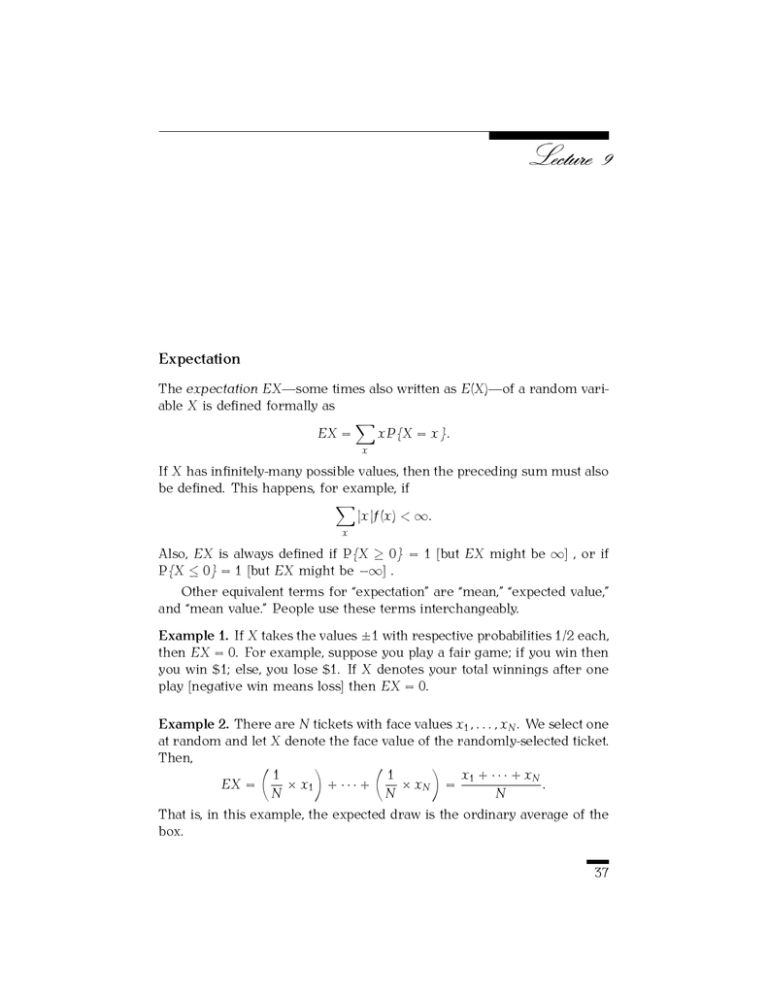
The expectation EX—some times also written as E(X)—of a random variable X is defined formally as
!
EX =
xP{X = x}.
x
If X has infinitely-many possible values, then the preceding sum must also
be defined. This happens, for example, if
!
|x|f(x) < ∞.
x
Also, EX is always defined if P{X ≥ 0} = 1 [but EX might be ∞] , or if
P{X ≤ 0} = 1 [but EX might be −∞] .
Other equivalent terms for “expectation” are “mean,” “expected value,”
and “mean value.” People use these terms interchangeably.
Example 1. If X takes the values ±1 with respective probabilities 1/2 each,
then EX = 0. For example, suppose you play a fair game; if you win then
you win $1; else, you lose $1. If X denotes your total winnings after one
play [negative win means loss] then EX = 0.
Example 2. There are N tickets with face values x1 , . . . , xN . We select one
at random and let X denote the face value of the randomly-selected ticket.
Then,
"
#
"
#
1
1
x1 + · · · + xN
EX =
× x1 + · · · +
× xN =
.
N
N
N
That is, in this example, the expected draw is the ordinary average of the
box.
37
38
9
Example 3 (Constant random variables). Every number c is a random
variable [P{c = x} = 0 if x &= 0, and P{c = c} = 1]. Therefore, Ec = c.
Example 4 (Indicators). Let A denote an event, and form a random variable
IA by setting IA := 1 if A occurs, and IA := 0 otherwise. Note P{IA = 1} =
P(A) and P{IA = 0} = P(Ac ). Therefore,
E(IA ) = P(A).
Theorem 1 (Addition rule for expectations). Suppose X and Y are random
variables, defined on the same sample space, such that EX and EY are
well defined and finite. Then, for all constants α and β,
E(αX + βY ) = αEX + βEY .
Proof. If we could prove that
E(cZ) = cE(Z)
(10)
for every constant c and random variable Z. Then, αEX = E(αX) and
βEY = E(βY ). Therefore, we would have to show that E(X ' + Y ' ) = E(X ' ) +
E(Y ' ) where X ' := αX and Y ' := βY . That is, (10) reduces the problem to
α = β = 1.
In order to prove (10) we compute:
$
!
!
x%
E(cZ) =
xP{cZ = x} =
xP Z =
c
x
x
%
! &x ' $
x
=c
P Z=
.
c
c
x
Change variables [u := x/c] to find that
!
E(cZ) = c
uP{Z = u} = cEZ,
u
as asserted.
It remains to prove the theorem with α = β = 1. First of all note that
!
!
P{X + Y = a} =
P{X = b , Y = a − b} :=
f(b , a − b).
b
b
[f denotes the joint mass function of (X , Y ).] Therefore,
!
! !
E(X + Y ) =
aP{X + Y = a} =
a
f(b , a − b).
a
a
b
Expectation
We can write a as (a − b) + b and substitute:
!
!
!!
E(X + Y ) =
(a − b)
f(b , a − b) +
bf(b , a − b) .
(
a
b
)*
+
T1
(
a
b
)*
T2
39
+
In order to compute T1 , we change the label of the variables [c := a − b]:
!
! !
c
f(b , c) =
cP{Y = c} = EY .
T1 =
c
( b )*
+
marginal of Y
c
As regards T2 , we reorder the sums first, and then relabel [c := a − b]:
! !
! !
!
T2 =
b
f(b , a − b) =
b
f(b , c) =
bP{X = x} = EX.
b
a
The theorem follows.
b
( c )*
+
marginal of X
b
!
The addition rule of expectation yields the following by induction:
Corollary 1. If X1 , . . . , Xn are all random variables with well-defined
finite expectations, then
E(X1 + · · · + Xn ) = EX1 + · · · + EXn .
Example 5 (Method of the indicators). The “method of the indicators” is
an application of the previous example and the previous corollary in the
following way: If A1 , . . . , AN are events, then
E (IA1 + · · · + IAN ) = P(A1 ) + · · · + P(AN ).
You should note that IA1 + · · · + IAN denotes the number of events among
A1 , . . . , AN which occur.
We will make several uses of the method of the indicators in this
course. The following is our first example.
Example 6 (The mean of the binomials). Let X have the binomial distribution with parameters n and p. What is EX? Of course, we can use the
definition of expectations and write
" #
n
!
n k
EX =
k
p (1 − p)n−k .
k
k=0
But this is not a simple-to-understand expression. Here is a more effective approach: We can realize X = IA1 + · · · + IAn where A1 , . . . , An are
independent events with P(A1 ) = · · · = P(An ) = p. In particular,
EX = P(A1 ) + · · · + P(An ) = np.
40
Thus, for example, in 10 tosses of a fair coin we expect np = 10 ×
heads.
Example 7. For all constants a and b, and all random variables X,
1
2
9
=5
E(aX + b) = aE(X) + b,
provided that EX is well defined. For instance, suppose the temperature
of a certain object, selected on a random day, is a random variable with
mean 34o Fahrenheit. Then, the expected value of the temperature of the
object in Celsius is
5
5
10
× (EX − 32) = × (34 − 32) =
.
9
9
9
Sort out the details.
Finally, two examples to test the boundary of the theory so far.
Example 8 (A random variable with infinite mean). Let X be a random
variable with mass function,

 1
if x = 1, 2, . . .,
P{X = x} = Cx 2
0
otherwise,
/
2
where C = ∞
j=1 (1/j ). Then,
But P{X < ∞} =
/∞
EX =
j=1 1/(Cj
2)
∞
!
j=1
= 1.
j·
1
= ∞.
Cj 2
Example 9 (A random variable with an undefined mean). Let X be a random with mass function,

 1
if x = ±1, ±2, . . .,
P{X = x} = Dx 2
0
otherwise,
/
where D = j=±1,±2,··· (1/j 2 ). Then, EX is undefined. If it were defined,
then it would be




−1
n
−1
n
!
!
!
!
j
j 
1
1
1
lim 
+
=
lim 
+
.
2
2
n,m→∞
n,m→∞
D
j
j
Dj
Dj
j=−m
j=1
j=−m
j=1
But the limit does not exist. The rough reason is that if N is large, then
/N
j=1 (1/j) is very nearly ln N plus a constant (Euler’s constant). “Therefore,”
Expectation
if n, m are large, then


−1
n
&n'
!
!
1
1

+
≈ − ln m + ln n = ln
.
j
j
m
j=−m
j=1
41
If n = m → ∞, then this is zero; if m * n → ∞, then this goes to −∞; if
n * m → ∞, then it goes to +∞.