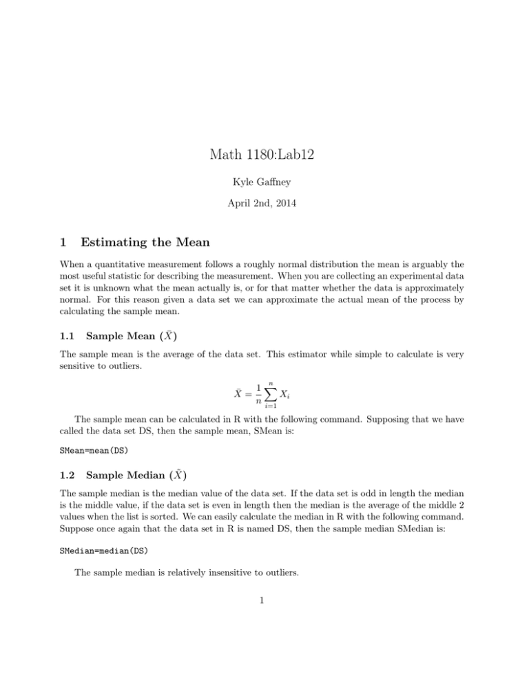
Math 1180:Lab12
Kyle Gaffney
April 2nd, 2014
1
Estimating the Mean
When a quantitative measurement follows a roughly normal distribution the mean is arguably the
most useful statistic for describing the measurement. When you are collecting an experimental data
set it is unknown what the mean actually is, or for that matter whether the data is approximately
normal. For this reason given a data set we can approximate the actual mean of the process by
calculating the sample mean.
1.1
Sample Mean (X̄)
The sample mean is the average of the data set. This estimator while simple to calculate is very
sensitive to outliers.
n
1X
X̄ =
Xi
n
i=1
The sample mean can be calculated in R with the following command. Supposing that we have
called the data set DS, then the sample mean, SMean is:
SMean=mean(DS)
1.2
Sample Median (X̃)
The sample median is the median value of the data set. If the data set is odd in length the median
is the middle value, if the data set is even in length then the median is the average of the middle 2
values when the list is sorted. We can easily calculate the median in R with the following command.
Suppose once again that the data set in R is named DS, then the sample median SMedian is:
SMedian=median(DS)
The sample median is relatively insensitive to outliers.
1
1.3
Trimmed Mean (X̄tr(k) )
The trimmed mean removes the largest and smallest k percent of the values and then calculates
the mean of the remaining set. By doing this you remove any outliers. It is very important to note
when one is using a trimmed mean as well as some form of justification as to why it was acceptable
to remove these values. When improper or fabricated results are created it is often due to improper
use of the trimmed mean. It turns out that R can calculate the trimmed mean for us with a simple
change to the arithmetic mean command we used for sample mean. If our data set is called DS
then the trimmed mean TMean is:
TMean=mean(DS,trim=.1)
This will give the trimmed mean with the smallest and largest 10 percent of the data set cropped
out.
2
Why must the Data be roughly normal?
Suppose that we generate a random data set from the exponential distribution. Recall that the
exponential distribution describes the time it takes a molecule to leave a cell. If an event occurs
with a probabilistic rate of 1/sec then the PDF of the exponential distribution will be f (t) = e−t ,
and the CDF will be F (t) = 1 − e−t . The expected value (or mean) of the exponential distribution
with rate=1 is Mean=1.
Let us simulate a random data set of this process in R.
DS=rexp(100,1)
SMean=mean(DS)
SMedian=median(DS)
Tmean=mean(DS,trim=.1)
summary(DS)
How did this compare to the actual value of the mean?
Now suppose that the rate is 10/sec (the mean of this process is
1
10 )
DS2=rexp(100,10)
SMean2=mean(DS2)
SMedian2=median(DS2)
TMean2=mean(DS2,trim)
summary(DS2)
How well did the data set compare to the exact mean of the process this time? Can you explain
why it performed that way?
2
3
Sample Variance and Standard Deviation
The sample variance is calculated as follows:
n
P
(xi − X̄)
n
P
x2i − nX̄ 2
= i=1
(1)
n−1
n−1
then the standard deviation of the data set is s, the square root of the variance.
Like most things this is simple to calculate in R, if our data set is named DS, then the standard
deviation of DS is:
s2 =
i=1
s=sd(DS)
4
Calculating the Confidence Limits
Suppose that we do not know the mean or the standard deviation of the process governing our
experiment (a pretty common assumption). We would like to find a confidence interval for the true
mean all the same. In other words we would like to find a confidence interval based off of our data
set so that we can say with some confidence that the true parameter value lies within this range.
The 95 percent confidence interval of the mean is:
s
µl = X̄ − 1.96 √
n
s
µh = X̄ + 1.96 √
n
The 99 percent confidence interval of the mean is:
s
µl = X̄ − 2.576 √
n
s
µh = X̄ + 2.576 √
n
Where X̄ is the sample mean, and s is the sample standard deviation. NOTE: this method
of finding the confidence interval should really only be used if n is greater than or equal to 30.
The reason for this stems from the fact that both the mean and the standard deviation were
both calculated from the data set which may or may not be generated from a perfectly normal
distribution.
3
4.1
Student’s T Distribution (for when n < 30)
The calculation of the confidence limits when n < 30 is similar, however it is necessary to pick
the values that we multiply the standard error ( √sn ) by from the critical values table of the T
distribution. For example when the degree of freedom (n-1) is 9 the equation for the 95 percent
confidence limits is:
s
µl = X̄ − 2.262 √
n
s
µh = X̄ + 2.262 √
n
Notice that this will result in a wider confidence range then if we could use the confidence limits
calculated from the normal distribution.
5
Assignment for the Week
1. Suppose that you are given the following data set tracking population changes do to immigration:
A=c(0,-1,1,1,-1,-1,1,2,0,0,-1,-1,-1,-1,-1,0,-1,1,-1,0)
Find the sample mean, the 10 percent trimmed mean, the median, and the standard deviation
for the data set in R.
2. This data set was calculated from the following probability distribution:
P r(−1) = 0.4
P r(0) = 0.2
P r(1) = 0.3
P r(2) = 0.1
Calculate the exact mean (expected value) and the exact variance and standard deviation for
this probability distribution.
3. Find the 95 percent confidence interval around the mean of the data set using the exact standard deviation calculated in the previous problem. Does the true mean lie in this confidence
interval?
4
4. Find the 95 percent confidence interval around the mean of the data set using the sample standard deviation you calculated in the first problem. Does the true mean lie in this confidence
interval?
Note: Just use the formula from the normal distribution (although technically it would be
safer to use the t-distribution)
5