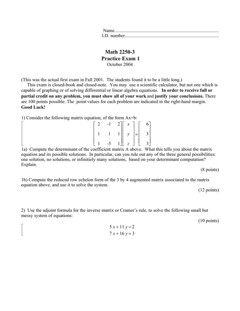
Name.........................................................................................
I.D. number................................................................................
Math 2250-3
Practice Exam 1
October 2004
(This was the actual first exam in Fall 2001. The students found it to be a little long.)
This exam is closed-book and closed-note. You may use a scientific calculator, but not one which is
capable of graphing or of solving differential or linear algebra equations. In order to receive full or
partial credit on any problem, you must show all of your work and justify your conclusions. There
are 100 points possible. The point values for each problem are indicated in the right-hand margin.
Good Luck!
1) Consider the following matrix equation, of the form Ax=b:
-1 2  x   6
 2

 



 


  y  =  3
 1
1
1

 



 



 


-5 1  z   3
 1
1a) Compute the determinant of the coefficient matrix A above. What this tells you about the matrix
equation and its possible solutions. In particular, can you rule out any of the three general possibilities:
one solution, no solutions, or infinitiely many solutions, based on your determinant computation?
Explain.
(8 points)
1b) Compute the reduced row echelon form of the 3 by 4 augmented matrix associated to the matrix
equation above, and use it to solve the system.
(12 points)
2) Use the adjoint formula for the inverse matrix or Cramer’s rule, to solve the following small but
messy system of equations:
(10 points)
5 x + 11 y = 2
7 x + 16 y = 3
3) Consider the differential equation
dP
2
=P −2P
dt
which could be a model for a certain population problem.
3a) Find the equilibrium solutions.
(5 points)
3b) Sketch the slope field for this differential equation. Onto the slope field sketch graphs of the
solutions to the four initial value problems with P(0)=-1, P(0)=0, P(0)=1, P(0)=2, P(0)=3. (You don’t
need formulas for the solutions to make the sketches!)
(10 points)
3c) Which of the equilibrium solutions are stable? Which are unstable?
(5 points)
3d) Which of population models we studied would lead to differential equation of this type? Be as
precise as you can, so that you account for the signs of both terms on the right of the differential
equation.
(5 points)
3e) Find a explicit solution to the initial value problem for this differential equation, with P(0)=3.
Explain what happens to your solution as time increases.
(15 points)
4) Consider the following configuration of two brine tanks: The first tank holds 200 gallons of water,
and the second tank holds 100 gallons. Solutions in each tank are well mixed so that each tanks’
concentration is uniform. Pure water flows into the first tank, at a rate of 10 gallons per minute; water
flows from tank 1 to tank 2 at the same rate, and water is removed from the second tank, also at the rate
of 10 gallons per minute.
4a) Assuming that the first tank initially contained a brine solution in which there was 1/2 pounds of salt
per gallon, explain why the amount of salt in this tank at time t minutes later is given by
x(t ) = 100 e
( −0.05 t )
(10 points)
4b) Let y(t) be the amount of salt in the second tank. Use the formula for x(t) from 4a, and your
modeling abilities to explain why y(t) satisfies the differential equation
(8 points)
dy
( −0.05 t )
+ 0.1 y(t ) = 5 e
dt
4c) Find the solution y(t) to the differential equation in 4b,, assuming the initial salt concentration in
tank 2 is also 1/2 pound per gallon.
(12 points)