wk11-13-06.nb
1
Consider a large population of sales figures. I've defined it to the computer with the name "popSALES. How may we learn
about this population? If we could manage to census the population we could easily obtain the mean and sd.
size@popSALESD
4000
Mean@popSALESD
14.7676
sd@popSALESD
9.3669
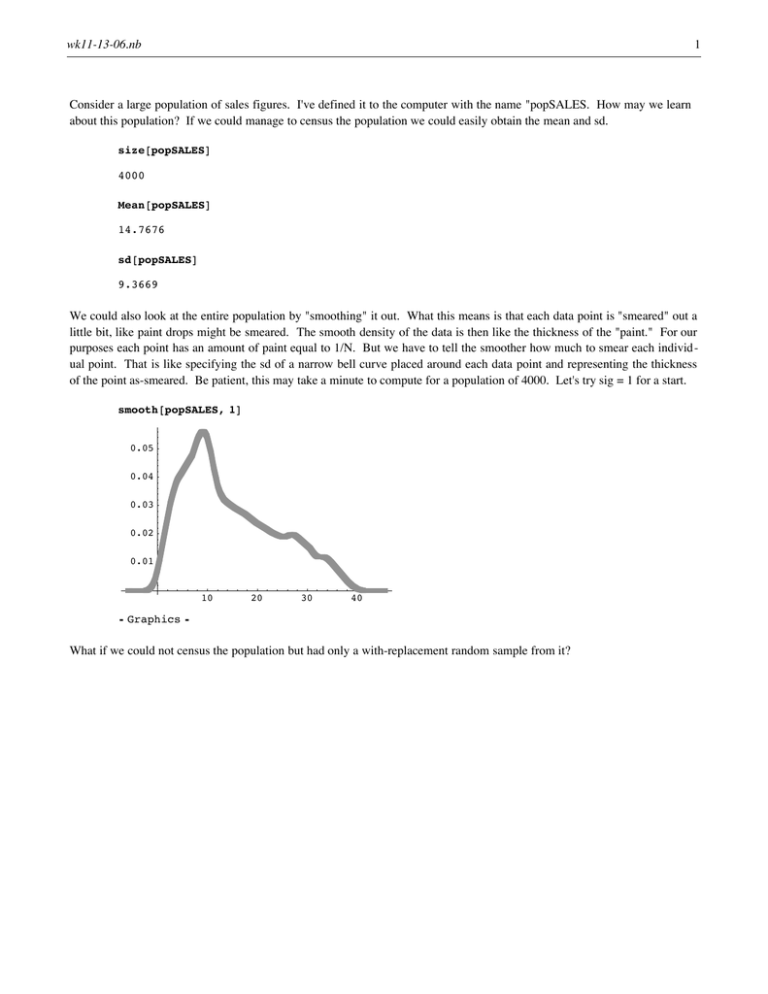
We could also look at the entire population by "smoothing" it out. What this means is that each data point is "smeared" out a
little bit, like paint drops might be smeared. The smooth density of the data is then like the thickness of the "paint." For our
purposes each point has an amount of paint equal to 1/N. But we have to tell the smoother how much to smear each individual point. That is like specifying the sd of a narrow bell curve placed around each data point and representing the thickness
of the point as-smeared. Be patient, this may take a minute to compute for a population of 4000. Let's try sig = 1 for a start.
smooth@popSALES, 1D
0.05
0.04
0.03
0.02
0.01
10
20
30
40
Ü Graphics Ü
What if we could not census the population but had only a with-replacement random sample from it?
wk11-13-06.nb
samSALES = sample@popSALES, 600D
2
811.85, 5.2, 14.52, 26.65, 24.76, 30.67, 27.65, 8.85, 10.9, 35.12, 9.09, 8.13, 24.56, 27.37,
14.21, 16.03, 6.18, 15.07, 32.56, 4.44, 19.56, 16.57, 4.17, 14.44, 10.32, 20.81, 2.09,
17.18, 10.25, 21.76, 8.87, 7.55, 24.11, 10.1, 14.06, 20.83, 11.33, 32.72, 34.59, 8.52,
11.67, 13.04, 9.47, 9.49, 22.63, 9.5, 19.65, 5.37, 14.91, 15.01, 10.07, 24.1, 8.54,
20.09, 11.55, 2.64, 27.45, 5.88, 18.75, 6.85, 3.52, 8.42, 10.96, 8.46, 19.05, 4.14,
23.64, 8.94, 7.71, 23.27, 1.4, 28.16, 11.75, 22.89, 0.51, 7.02, 4.25, 16.98, 7.71,
5.94, 8.78, 33.03, 12.06, 19.96, 21.86, 12.55, 3.49, 4.11, 36.87, 7.34, 16.41, 14.71,
14.8, 11.38, 13.69, 17.5, 15.07, 28.69, 19.35, 7.54, 14.03, 15.57, 7.97, 24.96, 9.79,
1.97, 24.25, 5.61, 32.6, 10.99, 10.21, 5.77, 22.55, 8.03, 3.01, 4.44, 5.04, 24.11,
4.67, 9.93, 14.99, 10.96, 29.25, 23.53, 3.62, 24.76, 2.17, 10.27, 17.8, 4.84, 35.99,
8.44, 31.12, 26.29, 4.95, 18.91, 2.02, 8.27, 28.69, 13.14, 3.24, 27.26, 11.29, 14.42,
16.71, 8.27, 3.76, 4.13, 8.72, 9.68, 12.63, 17.4, 7.49, 26.38, 30.7, 3.54, 2.95,
14.72, 8.53, 5.56, 26.77, 17.35, 24.29, 10.79, 9.65, 26.75, 8.71, 6.65, 8.03, 8.38,
25.87, 3.01, 9.1, 19.21, 34.05, 3.49, 29.64, 27.01, 10.43, 27.33, 13.85, 10.25, 27.01,
4.79, 6.67, 19.36, 5.13, 34.67, 9.76, 7.62, 27.61, 11.62, 26.8, 7.04, 19.88, 2.64,
19.66, 15.84, 17.05, 28.04, 24.56, 31.55, 22.28, 9.1, 7.34, 13.37, 9.57, 24.12, 5.39,
15.74, 5.76, 6.29, 33.53, 4.04, 10.48, 5.86, 19.78, 15.56, 15.44, 22.95, 28.47, 3.05,
24.98, 1.8, 27.39, 9.51, 1.99, 34.55, 10.28, 12.39, 6.79, 29.88, 13.96, 20.93, 19.18,
16.96, 27.03, 5.18, 7.49, 8.78, 2.06, 27.86, 26.89, 25.18, 19.65, 26.75, 30.3, 24.24,
0.28, 19.02, 7.33, 4.89, 8.69, 10.67, 16.15, 10.32, 1.94, 13.29, 15.89, 10.28, 5.4,
4.67, 2.91, 17.76, 20.44, 7.81, 2.35, 26.89, 12.55, 31.35, 1.8, 18.84, 37.24, 16.72,
13.3, 10.38, 2.38, 15.01, 20.38, 8.74, 13.7, 4.79, 17.43, 29.21, 16.59, 4.86, 28.96,
8.55, 8.27, 32.86, 12.46, 17.86, 7.97, 8.13, 5.14, 10.16, 11., 11.83, 0.48, 18.56,
11.22, 23.8, 25.21, 17.6, 4.11, 0.28, 10.79, 6.72, 6.52, 11.73, 7.86, 17.8, 9.82,
7.44, 11.31, 10.31, 9.16, 19.36, 34.79, 11.19, 8.15, 3.88, 7.33, 9.81, 10.49, 7.07,
27.3, 14.03, 15.75, 7.77, 11.88, 9.4, 7.71, 9.29, 8.83, 20.19, 16.92, 7.67, 18.01,
7.49, 16.92, 22.28, 14.08, 2.56, 10.69, 4.02, 17.43, 10.79, 13.21, 9.79, 31.72, 12.31,
6.56, 26.4, 5.48, 11.2, 34.89, 10.44, 9.95, 13.34, 3.1, 9.17, 5.69, 5.33, 8.76, 11.79,
24.93, 30.91, 2.64, 13.18, 20.54, 13.38, 8.14, 20.38, 23.07, 25.03, 16.21, 16.98,
33.7, 17.45, 35.75, 33.36, 6.12, 12.04, 25.42, 4.97, 26.06, 7.65, 3.29, 5.15, 17.46,
5.34, 22.2, 10.32, 7.18, 14.45, 14.42, 17.86, 1.69, 29.64, 10.01, 8.07, 23.77, 3.26,
32.56, 6., 24.02, 24.69, 7.51, 18.13, 5.22, 1.75, 14.34, 3.42, 6.3, 11.82, 12.04, 9.81,
18.36, 13.96, 14.42, 28.68, 7.86, 3.59, 4.04, 11.55, 3.54, 36.5, 32.91, 7.38, 4.55,
6.04, 11.22, 17.35, 3.68, 29.35, 9.98, 30.92, 13.77, 2.57, 22.5, 6.98, 19.61, 21.49,
4.04, 21.22, 1.25, 7.36, 22.17, 2.15, 9.88, 10.48, 28.2, 16.37, 3.84, 28.89, 15.36,
25.74, 3.9, 6.72, 16.46, 14.21, 12.35, 28.09, 8.03, 21.31, 10.33, 27.37, 20.72, 8.27,
2.09, 26.01, 17.63, 9.44, 14.92, 36.67, 15.25, 8.76, 26.02, 22.37, 21.06, 36.93, 3.56,
25.87, 3.59, 37.61, 15.12, 13.08, 13.28, 7.93, 20.81, 1.69, 35.25, 32.65, 6.47, 5.61,
20.69, 8.56, 18.7, 9.71, 5.84, 3.07, 10.84, 7.19, 6.88, 22.28, 31.48, 10.41, 17.15,
21.69, 1.29, 28.66, 8.16, 17.4, 15.01, 20.55, 7.5, 5.82, 32.38, 15.98, 6.88, 4.79,
36.2, 2.21, 2.22, 20.79, 1.69, 20.42, 11.77, 9.13, 9.85, 15.89, 4.15, 14.66, 27.73,
5.93, 13.94, 7.18, 6.21, 4.27, 5.93, 10.94, 30.33, 33.84, 20.93, 6.62, 3.43, 29.01,
7.16, 2.21, 8.08, 35.25, 8.37, 18.6, 24.56, 9.25, 3.07, 14.82, 20.72, 26.13, 6.47,
24.98, 11.3, 12.63, 20.11, 11.68, 7.83, 14.06, 3.86, 5.22, 15.19, 11.49, 28.23, 11.1,
5.54, 9.79, 11.79, 29.93, 3.1, 10.59, 26.75, 5.58, 14.25, 19.29, 5.69, 3.45, 8.03,
27.07, 12.11, 15.29, 12.25, 7.15, 12.64, 3.77, 9.05, 9.62, 13.45, 4.3, 8.13, 31.2<
Mean@samSALESD
14.3445
s@samSALESD
9.17597
wk11-13-06.nb
3
smooth@samSALES, 1D
0.05
0.04
0.03
0.02
0.01
10
20
30
40
Ü Graphics Ü
We can overlay the two graphics by citing their output line numbers in the command below. I may have different line
numbers than you will have. It will be seen that a sample of 600 has done a fairly good job of estimating the population
density.
Show@%16, %20D
0.05
0.04
0.03
0.02
0.01
10
20
30
40
Ü Graphics Ü
It is important to realize that the degree of smear obtained using sig = 1 in the above may not reveal the right degree of detail
about the population. If we lower sig, say to 0.5, we will get kinkier smoothings of both the population and the sample. But
if we press for too much detail the sample of 600 may not be able to reliably estimate that detail. When things work well we
choose a sig for which enough detail is provided and the reulting smoothing of the population is reliably estimated. It is
always a compromise and a "seat of the pants" decision just how to choose sig.
Here is a really small example of smoothing. The function "smooth2" puts the individual bell curves into view along with
their resulting density average. If you look carefully at the third picture you will see how it passes halfway between the two
normal curves. It has the average of their heights.
smooth2@810, 14<, 1D
wk11-13-06.nb
4
0.4
0.3
0.2
0.1
7.5
10
12.5
15
17.5
20
7.5
10
12.5
15
17.5
20
7.5
10
12.5
15
17.5
20
0.2
0.15
0.1
0.05
0.4
0.3
0.2
0.1
Ü Graphics Ü
Here is another example. By choosing sig too large we will oversmooth and lose all detail. In this case the resulting density
tells us there is only one central area containing the data but does not reveal how the data are spaced apart in there.
smooth2@81, 2, 3<, 2D
wk11-13-06.nb
5
0.2
0.15
0.1
0.05
-10
-5
5
10
15
5
10
15
5
10
15
0.175
0.15
0.125
0.1
0.075
0.05
0.025
-10
-5
0.2
0.15
0.1
0.05
-10
-5
Ü Graphics Ü
Reducing sig from 2 (just above) to 0.2 produces more detail, maybe too much.
smooth2@81, 2, 3<, 0.2D
wk11-13-06.nb
6
2
1.5
1
0.5
1
2
3
4
1
2
3
4
1
2
3
4
0.6
0.5
0.4
0.3
0.2
0.1
2
1.5
1
0.5
Ü Graphics Ü
CI. Here is a routine with which to do t (or z) based CI (the case of 0-1 data would be a little different because it uses
root(pHAT qHAT) instead of s, but they are almost the same when n is large). The CI routine takes data and t (oir z) and
reports
{mean, n, s, z (or t), CI}
ci@samSALES, 1.96D
814.3445, 600., 9.17597, 1.96, 813.6102, 15.0787<<