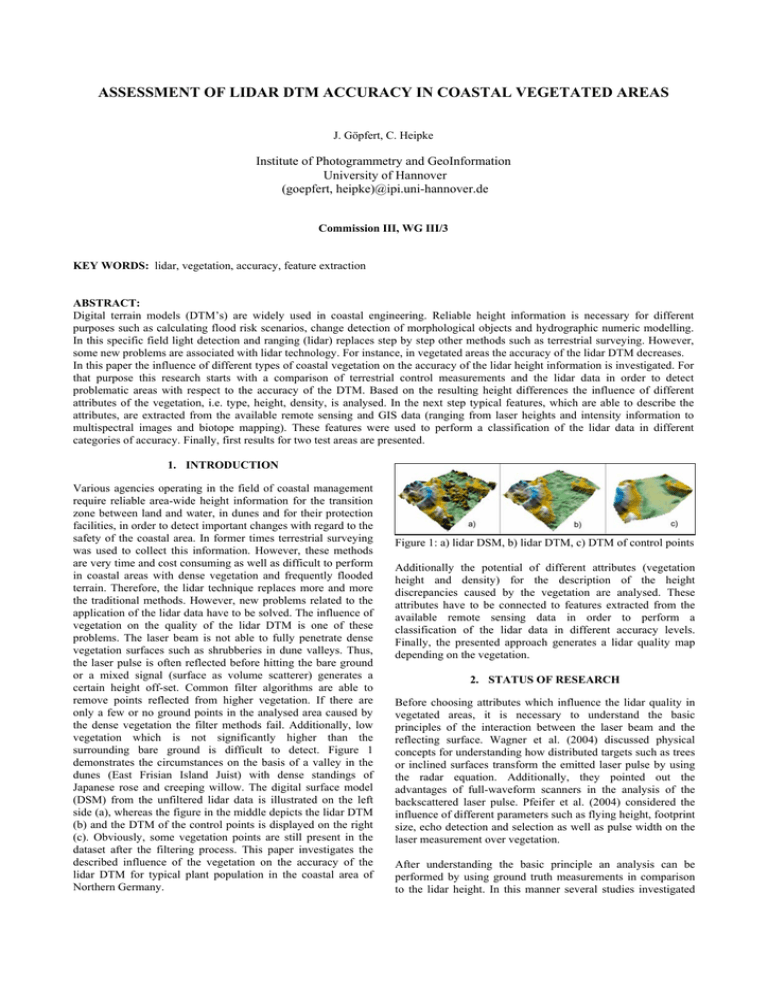
ASSESSMENT OF LIDAR DTM ACCURACY IN COASTAL VEGETATED AREAS
J. Göpfert, C. Heipke
Institute of Photogrammetry and GeoInformation
University of Hannover
(goepfert, heipke)@ipi.uni-hannover.de
Commission III, WG III/3
KEY WORDS: lidar, vegetation, accuracy, feature extraction
ABSTRACT:
Digital terrain models (DTM’s) are widely used in coastal engineering. Reliable height information is necessary for different
purposes such as calculating flood risk scenarios, change detection of morphological objects and hydrographic numeric modelling.
In this specific field light detection and ranging (lidar) replaces step by step other methods such as terrestrial surveying. However,
some new problems are associated with lidar technology. For instance, in vegetated areas the accuracy of the lidar DTM decreases.
In this paper the influence of different types of coastal vegetation on the accuracy of the lidar height information is investigated. For
that purpose this research starts with a comparison of terrestrial control measurements and the lidar data in order to detect
problematic areas with respect to the accuracy of the DTM. Based on the resulting height differences the influence of different
attributes of the vegetation, i.e. type, height, density, is analysed. In the next step typical features, which are able to describe the
attributes, are extracted from the available remote sensing and GIS data (ranging from laser heights and intensity information to
multispectral images and biotope mapping). These features were used to perform a classification of the lidar data in different
categories of accuracy. Finally, first results for two test areas are presented.
1. INTRODUCTION
Various agencies operating in the field of coastal management
require reliable area-wide height information for the transition
zone between land and water, in dunes and for their protection
facilities, in order to detect important changes with regard to the
safety of the coastal area. In former times terrestrial surveying
was used to collect this information. However, these methods
are very time and cost consuming as well as difficult to perform
in coastal areas with dense vegetation and frequently flooded
terrain. Therefore, the lidar technique replaces more and more
the traditional methods. However, new problems related to the
application of the lidar data have to be solved. The influence of
vegetation on the quality of the lidar DTM is one of these
problems. The laser beam is not able to fully penetrate dense
vegetation surfaces such as shrubberies in dune valleys. Thus,
the laser pulse is often reflected before hitting the bare ground
or a mixed signal (surface as volume scatterer) generates a
certain height off-set. Common filter algorithms are able to
remove points reflected from higher vegetation. If there are
only a few or no ground points in the analysed area caused by
the dense vegetation the filter methods fail. Additionally, low
vegetation which is not significantly higher than the
surrounding bare ground is difficult to detect. Figure 1
demonstrates the circumstances on the basis of a valley in the
dunes (East Frisian Island Juist) with dense standings of
Japanese rose and creeping willow. The digital surface model
(DSM) from the unfiltered lidar data is illustrated on the left
side (a), whereas the figure in the middle depicts the lidar DTM
(b) and the DTM of the control points is displayed on the right
(c). Obviously, some vegetation points are still present in the
dataset after the filtering process. This paper investigates the
described influence of the vegetation on the accuracy of the
lidar DTM for typical plant population in the coastal area of
Northern Germany.
Figure 1: a) lidar DSM, b) lidar DTM, c) DTM of control points
Additionally the potential of different attributes (vegetation
height and density) for the description of the height
discrepancies caused by the vegetation are analysed. These
attributes have to be connected to features extracted from the
available remote sensing data in order to perform a
classification of the lidar data in different accuracy levels.
Finally, the presented approach generates a lidar quality map
depending on the vegetation.
2. STATUS OF RESEARCH
Before choosing attributes which influence the lidar quality in
vegetated areas, it is necessary to understand the basic
principles of the interaction between the laser beam and the
reflecting surface. Wagner et al. (2004) discussed physical
concepts for understanding how distributed targets such as trees
or inclined surfaces transform the emitted laser pulse by using
the radar equation. Additionally, they pointed out the
advantages of full-waveform scanners in the analysis of the
backscattered laser pulse. Pfeifer et al. (2004) considered the
influence of different parameters such as flying height, footprint
size, echo detection and selection as well as pulse width on the
laser measurement over vegetation.
After understanding the basic principle an analysis can be
performed by using ground truth measurements in comparison
to the lidar height. In this manner several studies investigated
the influence of different vegetation types on the quality of the
lidar DTM. Elberink and Crombaghs (2004) found a systematic
upwards shift of up to 15cm for low vegetated areas (creeping
red fescue). Ahokas et al. (2003) evaluated the lidar accuracy
for asphalt (standard deviation 10 cm), gravel (4cm), grass
(11cm) and forest ground (17cm). Pfeifer et al. (2004)
investigated the influence of long dense grass (+ 7.3cm), young
forest (+ 9.4cm) and old willow forest (+ 11.6cm) on the
accuracy of lidar data. Hodgson and Bresnahan (2004) used the
horizontal coordinates of the irregularly distributed lidar points
for the measurement of the ground truth in order to avoid an
interpolation influence during the calculation of an error budget
for a lidar data set. They found a standard deviation of 17cm for
evergreen and 26cm for deciduous forest, however in contrast
to other studies only low shifts (-4,6 cm for evergreen, + 1,0cm
for deciduous) occurred.
Only a few researchers investigated object or data driven
parameters with an influence of the laser measurement except
the vegetation type. Hopkinson et al. (2004) presented a method
to identify the relationship between the standard deviation of
pre-processed laser heights (the ground elevation was
subtracted from the first and last pulse measurement) and
vegetation height itself for low vegetation (<1,3m). They found
the following expression,
vegetation height = 2.7 * standard deviation,
and determined the r.m.s.e. of the predicted vegetation heights
with 15cm. Pfeifer et al. (2004) and Gorte et al. (2005) used
also the variation of the laser heights in order to detect relations
to the height shift in low vegetated areas. Instead of the
standard deviation they defined texture parameters and showed
their potential for correction.
In (Moffiet et al., 2005) the capabilities of classified returns
(ground and vegetation, first, last and single pulse) as well as
the returned intensity were investigated to distinguish different
tree types. The authors pointed out that the average and the
standard deviation of the intensity values are affected by the
forest structure as well as the reflective properties of the
vegetation, whereas the information content of a single intensity
value is difficult to interpret.
In different studies a combination of height and multispectral
data is used in order to detect and classify vegetation types. For
example, Mundt et al. (2006) explored the potential of this
combination for mapping sagebrush distribution; and Straub
and Heipke (2001) determine tree hypothesis using geometric
and radiometric features from height and image data.
3. DATA
This research is mainly based on two test flights. Most of the
investigations were carried out using data collected by the
company Milan-Flug GmbH covering the region of the East
Frisian Island “Langeoog” in the leaf-off period (April 2005).
During the campaign a LMS Q560 system of the company
Riegl was used. Flying at a height of 600m the system provided
an average point density of 2.9 points/m2. The following data
were collected:
RGB – Orthophotos (resolution: 0,2 m)
maximum of three pulses per laser beam
unfiltered raw data (x, y, z, intensity)
points (x, y, z), separated into ground and vegetation
Supported by biologists various control areas for typical
vegetation types were defined. Within a few days of the flight
campaign ground truth data for these regions were collected
including the height of the ground and the vegetation as well as
a verbal description of the vegetation. For each of the following
vegetation types two test fields were chosen:
Japanese rose (Rosa rugosa) (vegetation heights up
to 1,3 m)
Beach grass (Ammophila arenaria) (<1,0m)
Crowberry (Empetrum nigrum) (<0,4m)
Creeping willow (Salix repens) (<1,6m)
Common seabuckthorn (Hippophaë rhamnoides)
(<1,4m)
Common reed (Phragmites australis) (<2,2m)
Sand couch grass (Agropyron pungens) (<0,5m)
Furthermore, two mixed habitats (rose/seabuckthorn (<2,6m)
and seabuckthorn/willow (<1,6m) were investigated.
Additionally, some fisheye photos taken from the ground to the
zenith were acquired in order to quantify the vegetation density
(Figure 3). Four bare ground areas in the immediate vicinity of
the vegetated test region were surveyed to check the general
quality of the data.
The data for the second test flight were collected during a
measurement campaign of the company TopScan with an
ALTM 2050 scanner from Optech covering the East Frisian
island Juist (March 2004). The flying altitude was 1000m and
the system provided an average point density of 2 points/m2.
The following data were used for the analysis:
CIR – Orthophotos (resolution: 0,2 m)
last pulse data
unfiltered raw data (x, y, z, intensity)
points (x, y, z), separated into ground and vegetation
A test area called “Dunes” consisting of 696 control points
within a mixed population of Japanese rose and willow was
surveyed in the same way as described above. Vegetation
heights of up to 2,8m occurred.
Finally, a biotope mapping performed on aerial photos taken in
2002 and 2003 with a HRSC-AX and a DMC camera was used
as input for the distinction of different predominant vegetation
types.
4. METHODS
In this paper we analyse the relationship between different
object as well as data driven features and the accuracy of the
lidar DTM in vegetated areas. We combine image, lidar and
GIS data to accomplish this task. In contrast to the above
mentioned work our aim is not to do vegetation classification
Initially, section 4.1 investigates the characteristics of
vegetation with respect to the lidar measurement. The next
section connects the analysed vegetation attributes to features
generated from remote sensing data. Finally, in 4.3 the
workflow to classify the lidar data into different accuracy levels
using the extracted features is discussed.
4.1 Characteristics of vegetation in lidar data
For an assessment of the influence of vegetation attributes on
the quality of the lidar height information we use ground truth
measurements. In order to compare directly terrestrial and lidar
data it is necessary to interpolate the heights obtained by one of
the methods from the surrounding measurements. One argument
for the interpolation of the lidar data is the higher point density
(~3 points/m2 in comparison to ~0.5 points/m2 for the ground
truth measurements). Additionally, the topographic features of
the surface are not reflected in the point distribution of the
terrestrial data due to the difficult measurement conditions, i.e.
dense vegetation and rough terrain. For these reasons we
compute a DTM from the filtered lidar data and interpolate the
lidar height information for the control points using their x- and
y-coordinates. Then the mean height discrepancies (lidar-DTM
minus reference height) and their standard deviation were
determined.
the rectification process see r. g. Schwalbe, 2005). The images
are segmented into vegetation and background using simple
thresholds which are calculated from the minima of the grey
value histogram. Finally, the correlation between the degree of
coverage and the height discrepancies is investigated.
Initially the height discrepancies (lidar DTM minus reference
height) depending on one parameter are analysed. The influence
of the following parameters is investigated:
vegetation type
vegetation height
vegetation density
Many related studies found that the surface type is one of the
crucial factors for the accuracy of the DTM derived from lidar
data (see also status of research). For that reason the first
parameter which has to be analysed is the vegetation type.
Laser pulses do not penetrate every layer of the vegetation in a
similar way. Therefore, the laser beam is very often reflected
above the bare ground or a mixed signal from ground and
vegetation returns to the scanner. Thus, an upwards shift for the
lidar heights is expected in vegetated areas. Caused by the
different structure the influence of several vegetation types on
the lidar accuracy should vary.
The research focuses on typical vegetation for coastal areas,
beginning with layers of biomass covering the ground in spring,
produced by felted mulch or bear leaves during winter times.
For example dense standings of beach grass and shrubberies in
dunes as well as common reed and sand couch grass in the
transition zone between land and water belong to the monitored
vegetation types.
The vegetation height is the next analysed parameter. With
higher vegetation the distance of the laser beam through the
different layers of organic material becomes longer. Therefore,
assuming a uniform vegetation structure in every layer the
probability that a part of the laser energy is absorbed or
reflected before reaching the ground is higher.
In order to investigate the influence of the vegetation height the
parameter is divided into regular intervals. The height
discrepancies at the control points are assigned to the related
interval. For every related interval the mean and the standard
deviation of the height shift are determined and plotted over the
vegetation height.
Subsequent, the influence of the vegetation density is studied.
The vegetation density can not be measured directly. Therefore,
suitable values which are able to describe the characteristics of
the vegetation density must be defined. One method to quantify
this parameter determines the ratio of the classified ground
points to all lidar points in the analysed test field. This idea
assumes that in dense vegetation less laser pulses penetrate the
canopy and more vegetation points are filtered. For that reason
a larger ratio implies a lower vegetation density and can
potentially act as an indicator for higher accuracies of the lidar
DTM. However, the filter result may be wrong, and thus the
definition of vegetation density breaks down in very dense
vegetation surfaces which are hardly penetrated by the Laser
beam.
The analysis of the fish eye photos offers another method to
define the vegetation density (figure 2). An algorithm to
calculate the coverage with organic material depending on the
zenith angle was developed based on the rectified image (for
Figure 2: Segmented fish eye photo (rosa rugosa)
Note that the term “dense vegetation” is also related to the size
of the lidar footprint: lasers with smaller footprints are able to
penetrate vegetation with higher density in a more undisturbed
way. The impact of the size of the lidar footprint on the
penetration rate, however, is not subject of this research.
Finally, the parameters vegetation height and density are also
analysed with respect to only one vegetation type, in order to
describe a more complex model of the influence of the
vegetation on laser heights.
4.2 Features for classification
In the next step features have to be determined which are able
to represent the vegetation attributes in the remote sensing data.
The mean value and the standard deviation of the multispectral,
lidar height and intensity channels and some texture parameters
derived from the co-occurrence matrix (i.e. contrast and
homogeneity) are investigated. The co-occurrence matrix
contains the spatial dependencies of the grey values for certain
directions and distances (see e. g. Haralick, 1979).
Considering one vegetation type we assume that the mean
values of the Normalized Difference Vegetation Index (NDVI)
correspond to the vegetation density: The leaf area index (LAI)
is one of the most important parameters for characterising the
structure of canopy. Many studies such as (Pandya, 2004) found
a strong positive correlation between the LAI and the NDVI
calculated from remote sensing data. Therefore, if the NDVI
increases, the amount of active organic material and the
vegetation density in the pixel should be higher. For the test
flight in the area of the island Langeoog the near infrared
channel is not available. Thus, the Degree of Artificiality (DoA)
as defined in (Niederöst, 2000) is used instead of the NDVI.
Next, we relate lidar intensity to vegetation density: Every layer
of the vegetation where the laser pulse is reflected decrease the
intensity value for the following echoes. For that reason a lower
intensity indicates a higher vegetation density under the
assumption of a similar reflectivity observing only one kind of
vegetation and the same beam direction. However, very dense
vegetation surfaces which can not be penetrated by the laser
pulse yield higher intensity values. But the cross section of the
illuminated area is not as homogeneous as the footprint hitting
bare ground. Therefore, the average returned intensity in
vegetated areas should be lower. Thus, for pre-defined
neighbourhoods we compute the mean and the average of the
lidar intensity (also motivated by Moffiet et al. 2005).
Furthermore, features have to be defined for the vegetation
height. On one side we can use the contrast of the height image
derived from the co-occurrence matrix to describe height
differences in the local neighbourhood of a pixel. A higher
contrast is equivalent to larger differences of grey values, and
we assume a correlation with higher vegetation. On the other
side for vegetation heights larger than 0.5m different pulses can
be detected by the Riegl scanner. In this case we use the
differences between the first and the last pulse of lidar raw data
to define the vegetation height.
Finally, instead of extracting features for the distinction of
different vegetation types we use the biotope mapping in order
to limit the research area to one predominant plant population.
calculated and transformed into an image, so that the grey
values correspond to the height discrepancies. This image is
segmented into different accuracy levels. These segments are
used as training areas for the classification.
In the last step the feature vectors derived for the training areas
and the segmentation are used to classify the lidar height data
into different levels of accuracy. In this paper the Euclidian
distance between the feature vectors is used to classify the
current segment. For this method the features are normalised to
the same overall value in order to weight the features equally.
5. RESULTS
The capabilities of extracted features to describe the
characteristics of the vegetation and their influence on the
accuracy of the lidar DTM are tested using the height
discrepancies at the control points.
4.3 Classification
Based on the different data sources (multispectral image, lidar
data, biotope mapping) a supervised classification is performed
in order to divide the lidar data into different levels of accuracy
depending on the predominant vegetation. Figure 3 depicts the
workflow of the classification.
5.1 Characteristics of vegetation in lidar data
The influence of the vegetation type on the lidar accuracy is
illustrated in figure 4. Obviously, the lidar DTM is higher than
the related control points for each vegetation type (8 – 24 cm).
This finding corresponds to the theoretical consideration that
laser pulses do not penetrate all vegetation. For each type the
standard deviation of a single measurement is only in the range
from 5 up to 15cm. The highest height shift was detected for
beach grass (+19.3cm), seabuckthorn (+18.4cm), sand couch
grass (+20.1cm) and the mixed area seabuckthorn/willow
(+23.2cm).
Figure 3: Classification workflow
A segment based approach for the classification was chosen in
order to consider the local neighbourhood of the laser pulse and
to define mean values and standard deviation as well as other
texture parameters.
Initially, a DSM is calculated using the unfiltered lidar data in
order to preserve texture information stemming from the
vegetation. Subsequently, this DSM is transformed to a
greyscale image in order to use the data in combination with the
multispectral images for an image based classification. The
same procedure is accomplished for the intensity values of the
returned laser pulses.
The segmentation is performed using a region growing method
applied to the low pass filtered lidar intensity image. Starting
with the local grey value minima as seed regions (corresponds
to areas with low lidar accuracy), the analysed pixel is assigned
to the current segment if the difference of the average grey
value of the segment and the grey value of the pixel is smaller
than a certain threshold.
Previous work indicates that the vegetation type is an important
factor for the accuracy of the lidar DTM and for the
applicability of the discussed features. Thus, the extension of
the segments and, consequently, the area of the following
classification are limited to one predominant vegetation type
using the borderlines of the biotope mapping.
Training areas are generated by using the height discrepancies
from the control points. For that purpose a difference model is
Figure 4: Height shift for different surface types
(Langeoog, Riegl scanner)
Figure 5 illustrates the accuracy of the lidar DTM depending on
the vegetation height. The relatively large discrepancies for the
vegetation heights of 0.5 – 1.0m are caused by the beach grass
belonging to this range. Various standings of beach grass
produce a height shift up to 0.38m. In contrast many values
obtained by the control area in the reed lead to lower
discrepancies in the diagram for vegetation heights between 1.7
and 2.0m. Due to the vertical plant structure without
ramifications in the leaf-off period the influence of the reed on
the quality of the lidar DTM is low. In summary, the diagram
demonstrates that the vegetation height without considering
other parameters does not suffice in order to describe the height
discrepancies in the vegetated areas.
However, considering only one vegetation type some plant
heights show a strong correlation with the height discrepancies
(see figure 6). Obviously, the filtering process influences these
dependencies. If some points of the higher vegetation are
filtered, the accuracy for the related interval increases.
increases the accuracy of the lidar result, it unfortunately also
renders lidar intensity less useful as an indicator for the lidar
DTM accuracy, because the darker points potentially belonging
to the upper vegetation are filtered out.
Figure 5: Height shift plotted over vegetation heights for all
vegetation types (Langeoog, Riegl scanner)
Figure 8: Height shift plotted over lidar intensity for beach
grass (Langeoog, Riegl scanner)
Figure 6: Height shift plotted over vegetation heights for beach
grass (Langeoog, Riegl scanner)
In figure 7 the correlation between the vegetation density
calculated from the fisheye images and the height discrepancies
is visualised. Only a low correlation (0.19) was found
considering all vegetation types. However, for several lower
vegetation types a high correlation was detected, e.g. for beach
grass and Japanese rose. Therefore, for certain vegetation types
the defined vegetation density seems to correspond to the height
shift. The two negative values are caused by some outliers
which occurred due to the filtering process, as was determined
by a detailed analysis of the data.
Figure 9: Height shift plotted over lidar intensity for Japanese
rose/willow (Juist, ALTM scanner)
Figures 10 and 11 illustrate the height discrepancies depending
on the DoA and NDVI. Only a low correlation (0.39 for beach
grass (DoA), 0.23 for Dunes (NDVI)) between the height shift
and the indices could be identified. Due to the fact that the
measurement campaign was conducted in spring, the plants in
the test area Dunes (rose, willow) had just started their activity.
Therefore, in general only low NDVI values occurred.
Obviously, the correlation for active vegetation such as beach
grass is higher.
Figure 7: Correlation between the degree of coverage of the
fisheye photos and the height shift (zenith angle up to 40°)
5.2 Features for classification
Figures 8 and 9 show the height discrepancies depending on the
lidar intensity for some vegetation types. A high negative
correlation can be detected for the intensity values (-0.51 for
beach grass, see figure 8), and especially for the lidar DSM (0.92 instead of -0.6 for the DTM, see figure 9). Thus, whereas
the filtering process eliminates higher vegetation and therefore
Figure 10: Height shift plotted over DoA for beach grass (island
Langeoog, Riegl scanner)
Due to the completely different size and form of the training
areas and the segments it is also possible to compare the
classification result within the training areas in order to assess
the applicability of the segmentation process and the
practicability of the classification using the extracted features.
A good match can be detected in the second example for the
test area Dunes (figure 13).
Table 2: Extracted features for the accuracy levels of the test
area Dunes (not normalised)
Figure 11: Height shift plotted over NDVI for the test area
dunes (Japanese rose/willow, island Juist, ALTM scanner)
Parameter
Area Height Shift (cm)
Class (Height Shift)
Mean Green
Mean NDVI
Mean Intensity
Height Contrast
<+15
84,7
129,0
88,5
0,28
Test Area Dunes
(-7,7) – (+72,0)
<+30
<+45
<+60
81,1
77,3
76,7
136,9
146,0
145,6
81,6
62,0
40,5
0,34
0,68
0,62
>+60
76,5
149,2
38,3
0,50
In summary, lidar intensity as well as vegetation indices show
potential for the distinction of different accuracy levels in the
lidar DTM. Additionally, a negative correlation between the
height shift and the values of the channels in the visible
spectrum was also detected. However, all values vary strongly
in a single accuracy interval. Therefore, mean values for
segments are more suitable for classification purposes.
5.3 Classification
Finally, first classification results for beach grass and the test
area Dunes are presented. Tables 1 and 2 summarise the
extracted features for different accuracy levels, while figures 12
and 13 illustrate the results graphically. In addition to the
features discussed in 5.2 the contrast of the height image was
also used (see also chapter 4.2).
In the first example two different training areas of beach grass
are used to classify the same region. If the algorithm works
correctly, the extracted features for the accuracy intervals in
table 1 and the classifications on the left and the right side of
figure 12 have to be the same. However, comparing these
features and classifications some differences can be identified.
The problems are associated with the different range of the
height shift (table 1 second row) and the varying size of the
control areas related to the accuracy levels for the two test
fields. The latter one has a strong influence on the extracted
height contrasts.
Table 1: Extracted features for the accuracy levels of beach
grass (not normalised)
Parameter
Area Height Shift (cm)
Class (Height Shift)
Mean Blue
Mean DoA
Mean Intensity
Height Contrast
Beach Grass 1
(+5,7) – (+34,5)
<+13
<+26
>+26
88,5
83,6
82,5
79,5
89,0
92,7
70,0
69,6
65,1
0,20
0,21
0,24
Beach Grass 2
(-1,2) – (+38,5)
<+13
<+26
>+26
86,4
83,0
80,6
76,1
89,2
94,5
83,6
67,7
60,8
0,13
0,30
0,33
Figure 13: Left: training area from control points, Right:
Classification result for a part of the island Juist (red = height
shift up to +15cm, green = +30cm, blue = +45 cm, cyan =
+60cm, pink = >+60cm)
6. CONCLUSION AND OUTLOOK
This paper discusses an approach for mapping the quality of
lidar heights in vegetated areas using a combination of various
data sources. Some features (lidar intensity, height contrast,
vegetation indices) show capabilities in order to classify lidar
data in vegetated areas into different accuracy levels. However,
attributes and features are strongly correlated to the vegetation
type. Therefore, a biotope mapping or a multispectral
classification of the vegetation has to be used in conjunction
with the lidar data.
The vegetation attributes, such as the height and density, as well
as some extracted features, such as lidar intensity, show a better
correlation to the height discrepancies using unfiltered lidar
data. Only the height contrast is related to the filtering process.
Therefore, the presented method should be applied to unfiltered
lidar data in order to assess the quality of the height information
in vegetated areas, and the filtering process has to be modelled
as well. For example, a simple method can be designed using a
difference model between the unfiltered and the filtered lidar
heights. This difference model can then be subtracted from the
predicted height shift.
The transferability of the features extracted from the lidar data
to other scanners, flight conditions and regions seems to be
difficult. For instance, lidar intensity values depend on many
parameters (i.e. the scanner type, echo detection methods and
intensity determination, characteristics of the emitted pulse,
flight date, surface type etc.). For the general transferability of
the method this approach uses ground truth data which adapt
the features to the current conditions.
ACKNOWLEDGMENTS
Figure 12: Classification result using two different control areas
of beach grass (red = height shift up to +13cm, green = +26cm,
blue = >26 cm)
This research has been financed by the Federal Ministry of
Education and Research (BMBF) under project no. 03KIS050.
We acknowledge the support of our project partners:
Department of Rural Area Husum (ALR), Federal Waterways
Directorate (WSD) and the Lower Saxony Water Management,
Coastal Defence and Nature Conservation Agency Division
Norden-Norderney (NLWKN).
Straub, B., Heipke, C. (2001): Automatic Extraction of Trees
for 3D-City Models from Images and Height Data. Automatic
Extraction of Man-Made Objects from Aerial and Space
Images. Vol. 3., eds. Baltsavias, Gruen, van Gool,
A.A.Balkema Publishers. Lisse Abingdon Exton(PA) Tokio. pp.
267-277.
REFERENCES
Schwalbe, E. (2005): Geometric Modelling and Calibration of
Fisheye Lens Camera Systems. The International archives of
Photogrammetry, Remote Sensing and Spatial Information
Sciences.Vol. XXXVI, Part 5/W8.
Ahokas, E., Kaartinen, H., Hyyppä, J.(2003): A quality
assessment of airborne laser scanner data. The International
Archives of Photogrammetry and Remote Sensing, Vol.
XXXIV, 3/W13, Dresden, Germany.
Gorte, B., Pfeifer, N., Oude Elberink, S. (2005): Height texture
of low vegetation in airborne laser scanner data and its potential
for DTM correction. The International archives of
Photogrammetry, Remote Sensing and Spatial Information
Sciences, Vol. XXXVI, Part 3/W19, pp. 150-155.
Haralick, R. M. (1979). Statistical and structural approaches to
texture. Proceedings of the IEEE 67(5), 786–804.
Hodgson, M. and P. Bresnahan (2004). Accuracy of Airborne
Lidar-Derived Elevation: Empirical Assessment and Error
Budget. Photogrammetric Engineering & Remote Sensing, Vol.
70, No. 3, March 2004, pp. 331-339.
Hopkinson, C., Lim, K., Chasmer, L.E., Treitz, P., Creed, I.F.,
Gynan, C. (2004): Wetland grass to plantation forest –
estimating vegetation height from the standard deviation of
lidar frequency distributions. The International archives of
Photogrammetry, Remote Sensing and Spatial Information
Sciences, Vol. XXXVI, Part 8/W2, pp. 288-294.
Moffiet, T., Mengerson, K., Witte, C., King, R., Denham, R.
(2005): Airborne laser scanning: Exploratory data analysis
indcates variables for classification of individual trees or forest
stands according to species. ISPRS Journal of Photogrammetry
& Remote Sensing 59 (2005), pp. 289-309.
Mundt, J. T., Streutker D. R., Glenn N.F. (2006): Mapping
Sagebrush Distribution Using Fusion of Hyperspectral and
Lidar Classifications. In Photogrammetric Engineering &
Remote Sensing, Vol. 72, No.1, January 2006, pp. 47-54.
Niederöst, M. (2000): Reliable Reconstruction of Buildings for
Digital Map Revision. The International Archives of
Photogrammetry and Remote Sensing, ISPRS, Amsterdam,
Netherlands, Vol. XXXIII, Part B3, pp. 635-642.
Oude Elberink, S. and M. Crombaghs (2004). Laseraltimetrie
voor de hoogtemetingen van de kwelders Waddenzee.
Technical Report AGI-GAP-2003-50 (in Dutch), AGI, RWS,
The Netherlands.
Pandya, M.R. (2004): Leaf Area Index Retrieval Using Irs Lissiii Sensor Data and validation of Modis Lai Product Over India.
The International Archives of Photogrammetry and Remote
Sensing, Vol. XXXV, Part B7, pp. 144-149.
Pfeifer, N., Gorte, B., Oude Elberink, S. (2004): Influences of
Vegetation on Laser Altimetry – Analysis and Correction
Approaches. The International archives of Photogrammetry,
Remote Sensing and Spatial Information Sciences, Vol.
XXXVII, Part 8/W2, pp. 283-287.
Wagner, W., Ullrich, A., Melzer, T., Briese, C., Kraus,
K.(2004): From single-pulse to full-waveform airborne laser
scanners: Potential and practical challenges. The International
Archives of Photogrammetry and Remote Sensing, Vol. XXXV,
Part B3, pp. 201-206.