COMBINING FULL SPHERICAL DEPTH AND HDR IMAGES
TO IMPLEMENT A VIRTUAL CAMERA
Axel Waggershauser
SpheronVR AG, Germany
awagger@web.de
February 22, 2005
KEY WORDS: Image Based Lighting, Point Clouds, Registration, Rendering, Light Probe, HDR
ABSTRACT:
Based on a real-world scene description consisting of N spherical depth images from a laser range scanner and M spherical (high
dynamic range) texture images we present a method that allows to place a virtual camera at an arbitrary position in the scene. The
proposed method considers the position and orientation of each depth and texture scan respectively to be unknown. A possible application is to “capture” background images or light probes for photorealistic rendering. The first step to achieve this goal is to register
the depth images relative to each other and mesh them, which is done by means of a combination of well known standard techniques.
The next step is to register the texture scans relative to the geometry. For this purpose, we developed an error model, based on image
coordinates of identified features in the depth and texture images, together with an appropriate minimization algorithm. The final step
of “capturing” the new image is implemented with a ray-tracing based algorithm. The capabilities and remaining problems of this
approach are discussed and demonstrated with high resolution real-world data.
1
0
INTRODUCTION
Creating photorealistic images or film sequences with both a realworld background and computer generated and animated objects
is a very common task in most of todays film productions in the
entertainment and advertising industry. This task needs the following entities of information: a) the background image, b) a
full description of the artificial object, including geometric and
reflectance (BRDF) properties, c) a complete description of the
lighting situation at the position in 3-dimensional space where
the artificial object should be inserted, i.e. what light (color and
intensity) comes from which direction, and d) geometry information of, at least, the immediate surrounding area around the position where the artificial object should be inserted and according
BRDF information for this geometry.
ϑ
π
0
2π
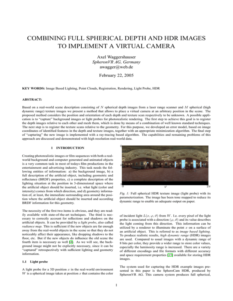
Fig. 1: Full spherical HDR texture image (light probe) with its
parameterization. The image has been tone mapped to reduce its
dynamic range to enable an adequate output on paper.
The necessity of the first two items is obvious, and they are readily available with state-of-the-art techniques. The third is necessary to correctly account for reflections and shadows on the
artificial objects. It can be provided by a light probe, also called
radiance map. This is sufficient if the new objects are far enough
away from the real-world objects in the scene so that they do not
noticeably affect their appearance, like dropping shadows to the
floor, etc. But if the new objects do influence the old scene the
fourth item is necessary as well [4]. As we will see, the background image might not be explicitly necessary, since it can be
“captured” retrospectively with sufficient lighting and geometry
information.
1.1
ϕ
of incident light L(x, ϕ, ϑ) from W . I.e. every pixel of the light
probe is associated with a direction (ϕ, ϑ) and its value describes
the light coming from this direction. This information can be
utilized by a renderer to illuminate the point x on a surface of
an artificial object. This is referred to as image based lighting.
To produce realistic results, high dynamic range (HDR) images
are used. Compared to usual images with a dynamic range of
8 bits per color, they provide a wider range to store color values,
especially the luminosity range is increased. There are a variety
of different encodings and file formats with different accuracy
and space requirement properties [15] available for storing HDR
images.
Light probe
The system used for capturing the HDR example images presented in this paper is the SpheroCam HDR, produced by
SpheronVR AG. This camera system produces full spherical,
A light probe for a 3D position x in the real-world environment
W is a spherical image taken at position x that contains the color
1
0
y
ϑ
y
x
ϑ
ϕz
x
π
0
Fig. 2: A light probe taken in x cannot be used in y. Some parts
of the light probe that are visible in point x should not be in y,
for example the highlighted section of the wall.
2π
Fig. 3: Full spherical depth image with its parameterization and
its associated local left hand coordinate system. The brighter the
image pixel is, the further away is the respective object. The
displayed range is approximately 1m to 25m.
1.3
high resolution HDR images in one shot. The image resolution
is up to 50 mega pixels and the dynamic range goes up to 26 bits
per color component. An example image is shown in fig. 1. Other
means to produce HDR light probes and HDR images in general
are presented in [4] and [5].
Outline
The first step to achieve this goal is to register the depth images
relative to each other and mesh them which is done by means of a
combination of well known standard techniques, sketched in section 2. The next step is to register the texture scans relative to the
geometry. For this purpose we developed an error model, based
on image coordinates of identified features in the depth and texture images, together with an appropriate minimization algorithm
which is presented in section 3. The final step of “capturing” the
new image is implemented with a ray-tracing based algorithm,
sketched in section 4. The capabilities and remaining problems
of this approach are discussed and demonstrated with high resolution real-world data in the results section 5. Section 6 concludes
this work and gives an outlook on possible future activities.
The objective of this work is to provide a method that allows to
place a virtual camera at an arbitrary position in a real-world
scene and “capture” background images or light probes for this
position. This method is based on a real-world scene description consisting of N spherical depth images from a laser range
scanner and M spherical (high dynamic range) texture images.
Each image is captured at an unknown positions with unknown
orientation.
1.2
ϕ
Light probe restrictions
To correctly light the point x on a surface of an artificial object,
one needs to have a light probe for exactly this position. In practice, however, a light probe for position x can be used to light
positions in a region around x. The size and shape of this region depends on the geometry of the real-world scene. Fig. 2
illustrates the situation. The point y should not receive incident
light from the highlighted section of the wall. This prohibits the
usage of a light probe obtained at point x for lighting the point
y. So relatively small objects might be lightable with a single
light probe but the problem gets worse when an animation is to
be rendered where the object moves across a real-world scene. In
this case several light probes along the trajectory of the object are
necessary.
2
GEOMETRY RECONSTRUCTION
The goal of the geometry reconstruction performed by our approach is to be later on able to cast a ray from an arbitrary point
inside the scene towards an arbitrary direction and be able to tell
where that ray hits the surface of an object in the scene.
To accomplish this goal, the set of N “raw” spherical depth images has to be preprocessed. The value of each pixel in a depth
image is a real number giving the distance between the scanner
and the object that was hit by the laser. The coordinates of a pixel
together with the depth value and the projection characteristics
of the scanner define a 3D point in the local scanner coordinate
system. This way each depth image is associated with a 3D point
cloud (see fig. 3).
This work reduces the number of necessary “real” light probes
captured on site and allows to replace most of them with “virtual”
light probes by utilizing geometry information. By projecting a
light probe onto the scene’s geometry, a raytracer can easily determine which parts of the light probe to consider when lighting
a given point. In case the geometry and lighting information is
sufficiently detailed and complete it is possible to extract background images as well.
On the one hand, each of these point clouds is separately meshed
into a set of triangles, representing patches of the surfaces of the
objects in the scene. Each of those triangle meshes is then simplified to reduce the number of triangles. This is desirable to reduce the memory and computation time requirements of the subsequent rendering algorithm. On the other hand, a registration of
the point clouds is performed to find the relative orientation and
position of the individual scans. This results in a set of triangle
meshes, registered relative to each other.
A similar goal has been addressed already by [6] and [16]. Both
proposals utilized photogrammetrically extracted geometry resulting in coarse approximations, which in turn produced obvious graphical artifacts in the resulting images. We have high
resolution scans from the laser based depth measurement system
Imager 5003, manufactured by Zoller+Fröhlich, available, which
allow for an accurate and highly detailed geometry reconstruction
of the scene.
A comprehensive overview and comparison of the state of art
techniques regarding geometry reconstruction can be found in
several papers like [2, 3] and in the introductory part in [9].
2
two views, an obvious method is to pick a “central” view as M
and process the remaining ones one after another.
(scanner)
The registration is further subdivided into a coarse and a subsequent fine registration. This is necessary since the used (fine)
registration algorithms is basically a minimization algorithm for
some error function and tends to get stuck in local minimum,
hence, it needs a proper starting configuration provided as an initial value of R and t to find the global optimum. This is achieved
by the coarse registration or pre-alignment step.
(objects)
Fig. 4: Shown is a schematic 1D example scan including points
of each class. Red dots belong to class verge, blue to back edge,
yellow to front edge, and grey to surface.
2.1
Coarse Registration The used method simply performs multiple (fine) registrations with different, evenly distributed start configurations and picks the one that fits best. The decision which fits
best is based the error measure that the fine registration algorithm
tries to minimize.
Point classification
As a preparation, necessary for subsequent tasks like normal
estimation, meshing, and registration, a classification of each
pixel/point of the input images is performed. Based on itself
and its neighbors, each point is assigned to one of the following
classes:
This approach is especially viable in case of spherical depth images with a high overlap because then both images contain virtually the same geometry information, and then the translation
parameters t can be approximated by identifying the centers of
mass of both point clouds. Furthermore, the remaining 3 degrees of freedom (the orientation) are usually de-facto reduced
to 1 since the scanning device is usually always setup with its top
pointing upwards. So, a small number, e.g. 8, of equally distributed horizontal “starting positions” for the scanner suffice to
find the correct registration.
• invalid: These are pixels with no useful distance information (e.g. the scanner does not receive enough light to estimate the distance). This classification is given by the scanner software.
• verge: These are the pixels next to an invalid pixel, i.e. pixels that have at least one neighbor with no distance information.
An interesting approach to establish a proper pre-alignment,
which also works with non-full spherical scans, is based on so
called spin-images and was presented in [11].
• front/back edge: These are the pixels at the near/far side of
a local discontinuity, forming the edge/“shadow edge” of a
contiguous surface patch.
Fine Registration The fine registration algorithm used in our
implementation is a variant of the widely known iterative closest
point (ICP) algorithm. Many variants of the algorithm, originally
introduced by [1], have been proposed. A comparison of available methods with a focus on efficiency can be found in [12].
• surface: These are the “good” points on an objects surface.
They (should) constitute the biggest part of all points in the
scans.
For an illustration of the different classes see fig. 4. This classification is not necessarily one-to-one, e.g. there may be pixels
which are both front edge and back edge pixels at the same time.
The selection of corresponding point pairs in our ICP variant is
based on a heuristic incorporating point distance, estimated normals and the point classification. For detailed information about
the actual implementation see [14].
The motivation behind the two edge classes is to be able to distinguish between points that have neighbors all belonging to the
same surface patch and those that have neighbors belonging to
different surface patches.
2.2
The update of the registration is performed by the closed-form
solution for absolute orientation of a point set V with respect to
M in presence of correspondence information P ⊂ V × M as
given in [10]. Based on the point pairs in P , it calculates a rigid
transformation T that minimizes the summed squared distance
error
X
E(P ) =
kT (v) − mk2 .
(2)
Registration
Given is a (fixed) model point cloud M ⊂ R3 in the global or reference coordinate system WM and a depth image with the associated (variable) view point set V ⊂ R3 in the depth image’s local
coordinate system WV . Searched is the position and orientation
of V in the reference coordinate system, i.e. a rigid transformation T : R3 → R3 that maps the points in V from WV to WM ,
so that V best matches M. This function has 6 degrees of freedom, 3 translation and 3 rotation parameters. A straightforward
way to represent T is a 3 × 3 rotation matrix R and a 3-element
translation vector t with
T (p) = Rp + t.
(v,m)∈P
This method separates the problem of finding T into first finding
R then t. The first part is also used as a general purpose alignment
method in an error metric used in the texture registration method
in section 3.
2.3
Meshing
The meshing is quite straightforward, since the connectivity of
the points is already given through their neighborhood relationship in the depth image. The pattern used for connecting the
points is depicted in fig. 5. The only thing that has to be taken
care of is to not connect points that belong to different surface
(1)
When registering two views relative to each other, one of them
can simply be defined as the model M, so its local coordinate
system becomes the global coordinate system. With more than
3
both representations, like edges, holes, etc. A clearly viable but
also clearly cumbersome method is to manually establish these
correspondences with interactive viewer applications allowing to
pick and export coordinates. This is the way we gathered the data
for our experiments.
Usually, laser range scanner systems do not only record the distance to a measured point, but also the intensity of the incident
light, reflected by the surface of the measured object. Each pixel
in the resulting grey scale image of the scene corresponds to
one pixel in the associated depth image. This renders it possible in principal to automatically establish correspondences between features in the HDR texture images and the depth images
by using the grey scale image as the bridging element. The correspondence between features in the color and the grey scale image
may be established by means of image comparison, like the linear
correlation coefficient.
Fig. 5: Adjacent points in the depth image are connected to form
a triangle mesh. Points from different surface patches are not
connected. Red dots belong to class verge, blue to back edge,
yellow to front edge, and grey to surface.
patches. This is achieved by assuring a triangle does not contain
a back edge and a front edge point at the same time.
Another way to utilize the accompanying grey scale image is to
support the user in determining the landmark coordinates with
sub-pixel accuracy and reduced noise. The additional information provides the crucial advantage that features, not recognizable in the depth image, namely the texture of the surface, may
be recognizable in the grey scale image. This allows to select
landmarks on flat patches of an object’s surface. The distance of
a landmark from the scanner may then be determined with the
aid of a plane of best fit for the surrounding points. This may
reduce the influence of noise of the single depth pixels considerably. Additionally, the angle coordinates of the landmark may be
determined with sub-pixel accuracy by incorporating an appropriate comparison operator for the grey scale and color images.
Simplification The number of triangles in the created meshes
tend to become huge as the depth images may easily contain more
than 10 million points, and for each point there are approximately
two triangles in the generated mesh. For a typical scene, such a
mesh is heavily oversampled, i.e. large patches of adjacent triangles lie on a plane and may be adequately described by only a
view triangles. Therefore, a smaller set of triangles may be found,
that still adequately describes the surfaces in the scene.
The simplification method used in this work was introduced
in [8]. The reason, this approach was chosen, was mainly its
availability as source code in the QSlim package [7]. We were
able to reduce the number of triangles in our meshes by a factor
of e.g. 100, which reduced the memory usage of the rendering
application and increased its speed substantially.
3
3.2
Some close research regarding the problem of finding position
and orientation of a device by means of using position and bearing information of landmarks has been done in the context of autonomous mobile robot localization [13]. Most of these robots are
some kind of wheel-driven vehicles, so their freedom of movement is usually restricted to two dimensions, namely the ground.
Hence, the problem of localization is restricted to the plane,
where only three degrees of freedom have to be determined: two
for the position and one for the orientation. There are closed form
solution available for this restricted problem. Our need for a solution in 3D lead to the development of a non-linear optimization
algorithm for this purpose.
TEXTURE REGISTRATION
The goal of registering the texture scans is basically the same as
registering the geometry scans: find the position and orientation
of the texture camera in the model coordinate system WM . The
available input for solving this problem is the texture scan and
the generated geometry model of the scene. The desired output is
again a vector t ∈ R3 and a real 3 × 3 rotation matrix R, where
t gives the position of the texture camera and R its orientation
relative to the model coordinate system.
The algorithm used for solving this problem consists of two basic
steps:
The following will describe the used error function, mapping the
parameter space to the positive real numbers with a global minimum at the position in the parameter space that solves our problem and the algorithm that is capable of finding that minimum:
1. Selecting a number of so called landmarks, recognizable
in texture and geometry, and establishing correspondences
between each landmark’s texture coordinates (2D) and its
geometry coordinates (3D).
Error Function The input of step 2 is a list of N landmarks.
Each landmark is given by its world coordinates LG ∈ R3 and its
texture coordinates LT ∈ T = [0..w) × [0..h) with w the width
and h the height of the texture scan.
2. Finding position and orientation of the texture camera in the
world coordinate system that does not contradict the correspondences found in step 1.
Each texture image is assigned a local coordinate system the same
way as the depth images in section 2 (see fig. 1 and 3). This way,
the texture coordinates are assigned a direction, which may be
represented as a unit vector v ∈ R3 with kvk = 1. The (inverse)
projection, mapping a texture coordinate to a unit vector, will be
−1
denoted by P T : T → R3 .
These two steps have to be performed for every texture image.
3.1
Finding Position and Orientation
Establishing Texture – Geometry Correspondences
The texture-geometry correspondences are established by identifying features of the real-world scene that can be recognized in
4
An ordered set of unit vectors or the points on the unit sphere they
correspond to, respectively, is called a hedge hog in the following. Ordered means, each is assigned a label or number, allowing
to distinguish them. The i-th vector of a hedge hog H will be
denoted by the subscript Hhii . The hedge hog model builds the
fundamental base structure for the error function. The transformation of the texture coordinates of N landmarks into their unit
vector representation results in such a hedge hog, which will be
referred to as the texture hedge hog
n
o
−1
HT = v = P T (LT
(3)
i ) | ∀ 1 ≤ i ≤ N ,
where
LT
i
(a)
Fig. 7: Example of an error function. The texture hedge hog
HT = HG ((0.5, 0.5, 0.5)T ) is created at the center of the unit
cube, which contains 5 randomly placed landmarks. (a) shows 3
iso-surfaces. (b) shows the slab at z = 0.5 plus the rubber sheet
of that slab.
∈ T are the texture coordinates of the i-th landmark.
The error function is based on the idea that each position p ∈ R3
in the world coordinate system WM may be assigned a (geometry) hedge hog

ff
LG
i −p
HG (p) = v =
|∀1≤i≤N ,
(4)
G
kLi − pk
There is a faster and numerically more stable alternative which
becomes evident after a closer look at the used algorithm to find
A. In fact, the desired value e(p) results as a byproduct from the
calculation of A. Details are omitted here (see [14]). Fig. 7 shows
an example of the error function.
3
where LG
i ∈ R are the world coordinates of the i-th landmark.
The elements of HG (p) give the directions of all N landmarks
in the local coordinate system of p. This hedge hog HG (p) may
then be compared with the texture hedge hog HT to calculate
the error e(p) at p. Fig. 6 gives an example of the hedge hog
definition for 2 dimensions.
LG
2
After the optimal position t is found by minimizing e(p) – which
will be the subject of the next section – the optimal rotation matrix R, describing the orientation of HT in WM , is given already.
It is the error minimizing matrix A from equation (5).
LG
1
Error Function Minimization The non-linear optimization algorithm, used to find the optimal estimate for t by minimizing the
error function e: t = arg minp e(p), is an ad-hoc implementation
of the idea of the steepest descent approach. The general structure
of the algorithm is a loop which calculates successive estimates
tk+1 , based on the last estimate tk and the error function e, until a termination condition is reached. Given a current estimate
tk for t, the gradient ∆e is numerically evaluated at tk and used
to indicate where the next estimate tk+1 should be placed. The
steepest descent of e at tk is in direction
HG (p)
p
LG
3
LG
4
Fig. 6: A hedge hog HG (p) at position p is the ordered set of
unit vectors pointing from p to Li .
d(tk ) =
kHG (p)hii − AHT hii k2
(6)
The idea behind l is similar to the adaptive step-size control
in methods for solving differential equations, like the RungeKutta method. l is adjusted in each iteration of the algorithm.
The adjustment is based on the difference between d(tk ) and
d(tk+1 ). If the relative angle between d(tk ) and d(tk+1 ) is
above a threshold, which is checked by evaluating the dot product
d(tk ) ∗ d(tk + l · d(tk )) < 0.8, the current step size l was too
big. It is then halved and a new d(tk+1 ) is calculated. This is repeated until the threshold is exceeded. In case d(tk ) and d(tk+1 )
are sufficiently similar the step size may be increased to speed up
the convergence.
Motivated by the mentioned closed form solution for the problem in two dimensions, where position and orientation are found
successively, we searched for an error function allowing the same
separation in the 3D setup. This way, the parameter space for the
non-linear minimization would be reduced from 6 to 3, resulting
in a faster and more stable implementation. I.e. the error function has to be invariant with respect to the orientation of the hedge
hogs. Different functions with this property have been evaluated.
Best results have been obtained with the following error function:
N
X
−∆e(tk )
.
k∆e(tk )k
The next estimate tk+1 is then calculated by adding the vector
d(tk ), multiplied with a “step size” factor l, to tk : tk+1 = tk +
l · d(tk ).
The goal of finding the position t and rotation R of the texture
camera may be expressed with the introduced hedge hog model:
find t and R such that HG (t) = RHT .
e(p) =
(b)
The algorithm seems to be quite unselective regarding the start
value t0 in terms of finding the optimum value for t. Several experiments suggested that the error function has in general only
one local minimum, which leads to a guaranteed convergence
to the correct solution. This has not been proven, though. A
suggesting
start value is the centroid of the landmarks: t0 =
PN
G
1
i=1 Li .
N
(5)
i=1
where A denotes the rotation matrix, which minimizes the error
e(p). This is achieved by using the closed-form method already
mentioned in section 2, introduced in [10]. Thus, e(p) can be
evaluated by first finding A and then actually calculate the sum
of squared distances of equation (5).
5
ktk
1e-01
1e-02
1e-03
1e-04
1e-05
1e-06
1e-07
1e-08
3. Distribution of the landmarks: The most important aspect regarding the distribution of the landmarks is the coverage of the
texture images with landmarks, i.e. the field of view that contains
landmarks. The ability of the algorithm to come even close to
the correct solution vanishes if the field of view is narrowed too
much. A coverage of the sphere of less than about 15%, wich
corresponds to a field of view of about 45◦ , is insufficient. So the
landmarks should be “spread all over” the sphere.
1e-06 1e-05 1e-04 1e-03 1e-02 1e-01
σG
4
Fig. 8: Shown is the error ktk of the final estimation for t depending on the noise in LG
i . Displayed is the average, minimum,
and maximum of 100 test-runs.
RENDERING
To capture an image with the virtual camera, each pixel is processed separately with a ray-tracing method, one after an other.
To process one pixel one has to deeming the color of the light
that incidents into position x from direction d, where x are the
eye coordinates of the virtual camera given in the world coordinate system WM .
As the algorithm adjusts the step size l automatically during its
execution, the initial value is not of great importance.
The algorithm is supposed to find a (local) minimum of e. At
such a minimum, the gradient ∆e vanishes. Thus, the algorithm
terminates as soon as ∆e(tk ) < τ falls below a small threshold.
First of all, a short summary of the preprocessings’ results: The
geometry reconstruction step yielded N triangle sets Gi with associated rigid transformations TiG (p) = RiG (p) + tG
i , aligning
those sets with the reference coordinate system WM . The texture registration step yielded M rotation matrices RjT and positional vectors tT
j , describing the orientation and position of the
associated M texture images Tj in WM .
Analysis of the Algorithm The described algorithm has been
analyzed regarding its ability to find the correct solution for t
depending on the following properties:
1. the level of noise in the landmark coordinates,
To determine the color of the light engaging in x from direction
d, the ray x + rd, with r ∈ R+ ∪ {∞}, is intersected with all N
triangle sets TiG (Gi ).
2. the number of landmarks N , and
3. the distribution of the landmarks.
This yields N intersections ri . The case where x + rd does
not intersect any triangle in TiG (Gi ) is represented by ri = ∞.
Those N ri are very likely different. Due to incomplete geometries some of them might be infinite and the others are suspect
to registration errors and noise. From this contradicting set of
intersections a single value
The basic setup for all tests has been the same. Both algorithm
T
inputs (the geometry and texture coordinates LG
i and Li ) have
been synthesized. N landmarks were randomly placed on the
sphere with a radius of 10m. The input texture hedge hog has
been simulated by synthesizing it from the geometry at the origin:
HT = HG (0). Hence, the “correct” solution for t was always the
null-vector. This allowed for a simple measure for the quality of
the result: ktk. Each test has been repeated a number of times and
the average, the maximum, and the minimum value were used
for interpretation. The obtained results and further details on the
specific tests are presented in the following.
r̄ =
N
X
µi ri
(7)
i=1
is distilled by weighting the individual ri . Our current implementation simply picks the closes intersection: r̄ = arg mini ri .
Other weightings, incorporating more of the ri , might be used to
smooth the surfaces.
1. Level of noise in the landmark coordinates: The most dominant influence regarding the error in the algorithm output is noise.
Both inputs, the geometry and the texture landmark coordinates,
are subject to noise (scanning system and manual picking of coordinates). The noise has been simulated by adding a random
variable vector with Gaussian distributed length and equally distributed direction after the creation of HT to the geometry coordinates of the landmarks. Fig. 8a shows the error dependent on
the standard deviation σG of the length of the noise vector. The
number of landmarks used for this diagrams was N = 10. An expectable value for σG in real world data would be approximately
5mm. Randomizing HT gives equivalent results.
With r̄, the position of the light source pd = x+ r̄d of direction d
has been found. The next step is to determine its color cd . Therefore, pd is transformed into the local coordinate system of each
−1
of the M texture images with the inverse RjT and tT
j and then
projected into texture coordinates with the appropriate projection
function PjT : R3 → T for the respective texture camera:
pd → (xj , yj ) = PjT (RjT
−1
(pd − tT
j )) ∈ T .
(8)
Finally, cd is calculated by summing the weighted colors from
each texture image Tj at the respective coordinates:
2. Number of landmarks N : From the viewpoint of the user, the
number of (necessary) landmarks should be kept as low as possible, since they are provided manually. The test showed, that the
number should be at least 5. In the absence of noise, N is virtually insignificant. To double the precision one has to quadruple
N, unfortunately. This effectively prevents the compensation of
noise by increasing N .
cd =
M
X
νj Tj (xj , yj ) .
(9)
j=1
The most obvious constraint for the weights νj is that only those
images Tj with an unobstructed line of sight from their position
6
(window side)
tT
j to pd may contribute to cd (see fig. 9). If any object was between tT
j and pd , the pixel Tj (xj , yj ) has seen this object, not
the surface at pd . On account of this, for each texture Tj , the ray
T
tT
j + r · (pd − tS
j ) is tested for intersection with the complete triangle set G =
TiG (Gi ). If there was an obstacle, the weight
νj is set to 0. The other texture images might contribute to cd .
tT
2
(busts)
D3
T2
tT
1
D1 T1
x
D2
z
(chandelier)
tG
1
(table)
tG
2
(door side)
pd
x
Fig. 10: Floor plan of the Kaisersaal, including the positions of
the texture images T1,2 and the depth images D1,2,3 . The local
coordinate system of D1 is the model coordinate system. The
texture image of fig. 1 is T1 and the depth image in fig. 3 is D2 .
Fig. 9: Occlusions in texture images have to be considered in the
weighting process. The texture at tT
2 may not contribute to the
color of point pd , since it is occluded.
the texture of those small objects is crucial for lighting, which is
the case for the light bulbs of the chandelier in fig. 11c. For background shots, even the rope on the ground might be considered
distracting.
Different weightings have been tested. Using only the texture
closest to pd leads to the highest local resolution but produces
visible artifacts at the transition boundary (fig. 11f). Averaging
all valid textures blurs the result due to registration errors. Best
results have been obtained by weighting the textures proportional
to their reciprocal distance to pd raised to a power.
Insufficient texture registration precision: Other than the
first two items, which are rather a problem of inadequate input
than a problem of the proposed methods, this one applies to the
latter. The puniest error in the registration of the texture causes
visibly falsely positioned color information near edges of realworld objects (fig. 11e) and at seams where different textures are
blended (fig. 11f).
There are exceptional cases, which need special handling. If all
ri from equation (7) are equal to ∞ there is no intersection of
the ray x + rd with any triangle in the set G. For indoor scenes,
which we focused on, this usually means there was no depth scan
covering the respective geometry. In this case we simply set the
color cd to black (fig. 11a). A similar problem arises when a
proper position pd has been found but no texture information for
this point is available.
5
The answer to the question of where the virtual camera can be
placed relative to the captured real-world geometry depends on
the demand for the resulting quality. The closer one comes to
patches of missing or wrongly registered geometry and texture
features, the worse become the rendering results. For (nearly)
closed topologies, like an indoor room, it is obvious that only
positions inside the room are valid.
RESULTS
The presented example renderings in this work are based on depth
and HDR texture images captured in the Kaisersaal in the historic
city hall of Hamburg, Germany (fig. 10).
6
CONCLUSION
A method for combining depth and HDR texture images to implement a virtual camera has been presented. This allows to render
photorealistic sequences with moving objects inside real-world
scenes.
The images of fig. 11 show some example renderings, generated
with the proposed techniques. They reveal some serious quality
deficiencies:
Black holes: Missing geometry or texture information results
in black holes (fig. 11a). A simple workaround is to interpolate
those black pixels in the image with the surrounding non-black
pixels, as shown in fig. 11b. For lighting purposes this might be
satisfying, but in background images this is no satisfying solution
for large patches of missing information like the doorway. The
only real solution for this is to add more texture and geometry
scans, containing the missing information.
Remaining problems of the proposed method are in particular the
manual establishing of texture and geometry feature correspondences in the texture registration step. This is cumbersome and
error prone.
The presented approach has several open ends and space for further research:
Overlooked geometry: If certain real-world objects are to
small to be sufficiently sampled by the laser scanner to form representing triangle representations, they are missing in the geometry model. An example is the red barrier rope in fig. 11c. Sudden
depth changes near object edges pose problems to the laser scanner, too (fig. 11f). This leads to falsely positioned texture information. For lighting purposes, this is usually no problem, except
• improved texture-depth feature correspondence establishing by incorporating sub-pixel accuracy and averaging techniques to reduce noise
• support for non-full-spherical scans as input and
• better heuristics to deal with missing geometry and texture
information.
7
(a)
(c)
(e)
(b)
(d)
(f)
Fig. 11: The most obvious quality problems in the background shots are: missing geometry and texture information (a, b); overlooked
geometry (c, d); and insufficient texture registration precision (e, f).
Acknowledgements Thanks
to
the
courtesy
of
Zoller+Fröhlich, SpheronVR, and Professor Kersten –
Hochschule für Angewandte Wissenschaften Hamburg for
the sensor data this work has been based on and to Thomas
Kollig for his support during the creation of my thesis, which
this paper was based on.
[8] M. Garland and P. S. Heckbert. Surface simplification using
quadric error metrics. Computer Graphics, 31(Annual Conference
Series):209–216, 1997. 2.3
[9] A. Grün and D. Akca. Least squares 3d surface matching. In The ISPRS International Archives of the Photogrammetry, Remote Sensing
and Spatial Information Sciences, volume XXXIV 5/W16, 2004. 2
[10] B. K. P. Horn. Closed form solution of absolute orientation using unit quaternions. Journal of the Optical Society of America A,
4(4):629–642, April 1987. 2.2, 3.2
References
[11] A. Johnson and M. Hebert. Surface registration by matching oriented points. In Proc. Int. Conf. on Recent Advances in 3-D Digital
Imaging and Modeling, pages 121–128, 1997. 2.2
[1] P. Besl and N. McKay. A method for registration of 3-d shapes.
IEEE Transactions on Pattern Analysis and Machine Intelligence,
14(2):239–256, February 1992. 2.2
[12] S. Rusinkiewicz and M. Levoy. Efficient variants of the ICP algorithm. In Proceedings of the Third Intl. Conf. on 3D Digital Imaging
and Modeling, pages 145–152, 2001. 2.2
[2] R. J. Campbell and P. J. Flynn. A survey of free-form object representation and recognition techniques. Comput. Vis. Image Underst.,
81(2):166–210, 2001. 2
[13] I. Shimshoni. On mobile robot localization from landmark bearings. IEEE Transactions on Robotic and Automation, 18(6):971–
976, 2002. 3.2
[3] G. Dalley and P. Flynn. Pair-wise range image registration: a study
in outlier classification. Comput. Vis. Image Underst., 87(1-3):104–
115, 2002. 2
[14] A. Waggershauser. Photorealistic rendering from depth and hdr images. Diploma thesis. Technische Universität Kaiserslautern, 2004.
2.2, 3.2
[4] P. Debevec. Rendering synthetic objects into real scenes: Bridging
traditional and image-based graphics with global illumination and
high dynamic range photography. Computer Graphics, 32(Siggraph
’98 Proceedings):189–198, 1998. 1, 1.1
[15] G. Ward.
High dynamic range image encodings.
URL
http://www.anyhere.com/gward/hdrenc/hdr_
encodings.html. 1.1
[5] P. Debevec and J. Malik. Recovering high dynamic range radiance maps from photographs. Computer Graphics, 31(Siggraph ’97
Proceedings):369–378, 1997. 1.1
[16] M. Wicke. Photorealistic rendering from high dynamic range
panorama scans. Diploma thesis. Universität Kaiserslautern, 2003.
1.2
[6] P. Debevec, Y. Yu, and G. Boshokov. Efficient view-dependent
image-based rendering with projective texture-mapping. Technical
Report CSD-98-1003, 20, 1998. 1.2
[7] M. Garland. qslim 2.0. URL http://graphics.cs.uiuc.
edu/~garland/software/qslim20.html. 2.3
8