A First Tutorial
(version 1/15/03)
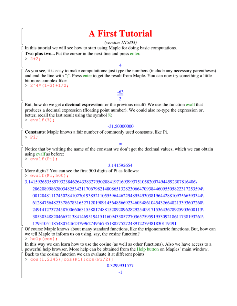
In this tutorial we will see how to start using Maple for doing basic computations.
Two plus two... Put the cursor in the next line and press enter.
> 2+2;
4
As you see, it is easy to make computations: just type the numbers (include any necessary parentheses)
and end the line with ";". Press enter to get the result from Maple. You can now try something a little
bit more complex like:
> 2^4*(1-3)+1/2;
-63
2
But, how do we get a decimal expression for the previous result? We use the function evalf that
produces a decimal expression (floating point number). We could also re-type the expression or,
better, recall the last result using the symbol %:
> evalf(%);
-31.50000000
Constants: Maple knows a fair number of commonly used constants, like Pi.
> Pi;
π
Notice that by writing the name of the constant we don’t get the decimal values, which we can obtain
using evalf as before:
> evalf(Pi);
3.141592654
More digits? You can see the first 500 digits of Pi as follows:
> evalf(Pi,500);
3.141592653589793238462643383279502884197169399375105820974944592307816406\
2862089986280348253421170679821480865132823066470938446095505822317253594\
0812848111745028410270193852110555964462294895493038196442881097566593344\
6128475648233786783165271201909145648566923460348610454326648213393607260\
2491412737245870066063155881748815209209628292540917153643678925903600113\
3053054882046652138414695194151160943305727036575959195309218611738193261\
17931051185480744623799627495673518857527248912279381830119491
Of course Maple knows about many standard functions, like the trigonometric functions. But, how can
we tell Maple to inform us on using, say, the cosine function?
> help(cos);
In this way we can learn how to use the cosine (as well as other functions). Also we have access to a
powerful help browser. More help can be obtained from the Help button on Maples’ main window.
Back to the cosine function we can evaluate it at different points:
> cos(1.2345);cos(Pi);cos(Pi/2);
0.3299931577
-1
0
Since a picture is worth a thousand words, we want to graph the sine function. For that we can use the
plot command as follows:
> plot(sin(x),x=-Pi..3*Pi);
Notice how we determine the range to be plotted. Go back to the previous line and modify the range
and, if you feel courageous, choose a different function.
1
0.5
–2
2
4
6
8
x
–0.5
–1
Problem: plot the fucntion cos(x^2) for x between 0 and 3*Pi.
>
Problem: plot the functions cos(2*x) and cos(x^2) for x between 0 and 3*Pi on the same graph. (
Suggestion: help(plot);).
>
Parametric plots are also obtained in a similar way. To graph a circle of radius 2 centered at (1,2) we
choose the parametric representation (2*cos(t)+1,2*sin(t)+2) and t between 0 and 2*Pi
> plot([2*cos(t)+1,2*sin(t)+2,t=0..2*Pi]);
4
3
2
1
–1
1
2
It is also possible to produce three dimensional graphics. For instance:
> plot3d((x^2+y^2),x=-2..2,y=-2..2);
3
Notice that by clicking anywhere on the previous graph you can rotate the image (that is, view the
graph from a different point).
Problem: rotate the previous graph so that you see the figure right from below.
>
>
An important tool is the use of variables. In the plotting example above we used the variables "x" and
"y", that didn’t have any preassigned value. But we can also store information in a variable:
> u:=7;
u := 7
Notice the use of the assignment operator ":=". To see the value of the variable "u" we simply type:
> u;
7
We can define our own functions:
> f:= x-> (x+1)^2-1;
f := x → (x + 1 )2 − 1
The evaluation works as expected:
> f(1);f(1.2345);f(x);f(u);f(7);
3
3.99299025
(x + 1 )2 − 1
63
63
Problem: define a function "myfunction" that maps x to x*exp(-x).
>
Among the many operations that Maple knows to manipulate polynomials we have
> simplify(f(x));
x2 + 2 x
Solving equations is also "easy":
> solve(f(x)=3,x);
1, -3
Maple knows about many areas of mathematics, but not all the specific knowledge is available all the
time. Some subjects have to be "loaded" into Maple’s memory. For that purpose we use the command
"with". Below we instruct Maple to load the Linear Algebra package:
> with(LinearAlgebra):
Notice that we have used ":" instead of the usual ";": this is so that the output of the command is
suppressed (you may want to go back, replace ":" by ";", type enter and see the difference).
Nothing seems to have happened. But now we can define "linear algebraic objects", like a Matrix:
> A:=Matrix([[1,2],[3,4],[5,6]]);
or, perhaps shorter,
> B:=<<3|2>,<5|6>,<-1|0>>;
2
 1




4
A :=  3




6
 5
2
 3




6
B :=  5




0
 -1
Problem: define a matrix C whose first columns has entries 3, 5.2 and Pi and whose second column
has entries -1, 0 and 1.
>
Vectors can be defined by
> v:=Vector([3,4,-1]);
 3




v :=  4




 -1
and, also, by:
> w:=<5,-4,3>;
 5




w :=  -4




 3
The components of a matrix or vector are addressed by:
> v[1];A[1,2];
3
2
We can also modify the components of a matrix or vector:
> v[1]:=-3;v;
v1 := -3
 -3




 4






-1


Operations on matrices are simple:
> A+B; 2*A; A-3*B;
4
 4




 8

10






6
 4
4
 2




 6

8






 10 12
 -8 -4




-12 -14






6
 8
We can solve linear systems of equations: consider the three equations:
> eqs := {a+b+2*c=6, 2*a+4*c=7, a+b/2+c=4};
b
eqs := {a + b + 2 c = 6, 2 a + 4 c = 7, a + + c = 4 }
2
One way of solving the system is using "solve" as before:
> solve(eqs,{a,b,c});
3
5
{c = , b = , a = 2 }
4
2
We can also look at the augmented matrix of the system:
> A:=<<1,2,1>|<1,0,1/2>|<2,4,1>|<6,7,4>>;
1
2
6
 1




 2

0
4
7

A := 




1

 1
1
4
2


We can find the reduced row echelon form of A by:
> ReducedRowEchelonForm(A);
where we can read again the solution of the linear system.
0
0
2 
 1






5
 0

1
0



2 





3 

 0
0
1

4 

The rank of a matrix is computed with the Rank command:
> Rank(A);
3
Problem: find the reduced row-echelon form and rank of the matrix C that you defined in a previous
problem.
>
We can also solve the following linear system where K is a constant.
> eqs2 := {a+b+2*c=6, 2*a+4*c=7, a+b/2+K*c=4};solve(eqs2,{a,b,c});
b
eqs2 := {a + b + 2 c = 6, 2 a + 4 c = 7, a + + K c = 4 }
2
5
3
7 K − 11
{b = , c = −
,a=
}
2
4 (K − 2 )
2 (K − 2 )
Notice that the solution is unique as long as K is not 2, where the solution doesn’t make sense. What
happens when K is 2? We start by substituting K=2 in the equations eqs2 and store the new equations
in eqs3. Then we solve.
> eqs3:=subs(K=2,eqs2);
> solve(eqs3,{a,b,c});
Notice that the solve command has no output, meaning that the system of equations has no solution.
b
eqs3 := {a + b + 2 c = 6, 2 a + 4 c = 7, a + + 2 c = 4 }
2
Alternatively, we can analyze the solutions using the reduced row echelon form:
> A:=<<1,2,1>|<1,0,1/2>|<2,4,2>|<6,7,4>>;
> ReducedRowEchelonForm(A);
1
2
6
 1




 2
0
4
7

A := 




1

 1
2
4
2


0
2
0
 1




 0
1
0
0





0
0
1
 0
The last expression confirms that the system is incompatible.
Yet another method for solving linear systems uses "LinearSolve" (use the help browser to get more
information). It can be used as follows:
> LinearSolve(A);
Error, (in LinearAlgebra:-LA_Main:-LinearSolve) inconsistent system
The error message shows once more that the system is inconsistent.
How about defining a linear transformation? Start by defining the coefficient matrix:
> C1:=<<1,-2,3>|<0,1,1>>;
0
 1




1
C1 :=  -2




1
 3
Applying C1 to a vector v is done with
> v:=<1,2>;
> C1.v;
 1

v := 

 2
 1




 0






 5
Finally, we define a linear transformation with
> T1:=z->C1.z;
T1 := z → C1 . z
To evaluate T1 we simply type
> T1(v);
 1




 0






 5
Similarly we define another matrix C2 and the linear transformation T2:
> C2:=<<1,2,-1>|<0,2,0>|<4,-1,1>>;
> T2:=z->C2.z;
4
 1 0





C2 :=  2 2 -1




-1
0
1


T2 := z → C2 . z
Redefine the vector v:
> v:=<x,y>;
 x 

v := 

 y 
Now compute the composition:
> T2(T1(v));
13 x + 4 y




 −5 x + y 






 2x+y 
Problem: what is the matrix associated to the composition of T2 and T1?
>
Finally, we can compute the product of the matrices C1 and C2:
> C2.C1;
4
 13




 -5 1






1
 2
Problem: define three matrices M1, M2, M3, so that the products M1.(M2.M3) and (M1.M2).M3 are
defined. Check that both triple multiplications give the same answer.
>
Problem: see how a circle of radius 1 centered at the origin is deformed under different linear
transformations of the plane into itself.
>
Sometimes, after using Maple for a while you need to clear Maple’s memory. This is done with the
restart command. But beware! Everything will be erased...
> restart:
>