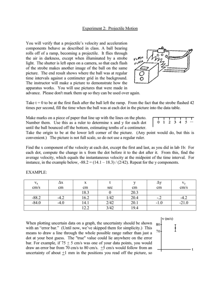
Experiment 2: Projectile Motion
You will verify that a projectile’s velocity and acceleration
components behave as described in class. A ball bearing
rolls off of a ramp, becoming a projectile. It flies through
the air in darkness, except when illuminated by a strobe
light. The shutter is left open on a camera, so that each flash
of the strobe makes another image of the ball on the same
picture. The end result shows where the ball was at regular
time intervals against a centimeter grid in the background.
The instructor will make a picture to demonstrate how the
apparatus works. You will use pictures that were made in
advance. Please don't mark them up so they can be used over again.
Take t = 0 to be at the first flash after the ball left the ramp. From the fact that the strobe flashed 42
times per second, fill the time when the ball was at each dot in the picture into the data table.
Make marks on a piece of paper that line up with the lines on the photo.
Number them. Use this as a ruler to determine x and y for each dot
until the ball bounced off the bottom, estimating tenths of a centimeter.
Take the origin to be at the lower left corner of the picture. (Any point would do, but this is
convenient.) The picture is not full scale, so do not use a regular ruler.
Find the x component of the velocity at each dot, except the first and last, as you did in lab 1b: For
each dot, compute the change in x from the dot before it to the dot after it. From this, find the
average velocity, which equals the instantaneous velocity at the midpoint of the time interval. For
instance, in the example below, -88.2 = (14.1 – 18.3) / (2/42). Repeat for the y components.
EXAMPLE:
vx
cm/s
Δx
cm
-88.2
-84.0
-4.2
-4.0
x
cm
18.3
16.2
14.1
12.2
t
sec
0
1/42
2/42
3/42
y
cm
20.3
20.4
20.1
19.4
When plotting uncertain data on a graph, the uncertainty should be shown
with an “error bar.” (Until now, we’ve skipped them for simplicity.) This
means to draw a line through the whole possible range rather than just a
dot at your best guess. The "true" value could lie anywhere on the error
bar. For example, if 75 + 5 cm/s was one of your data points, you would
draw an error bar from 70 cm/s to 80 cm/s. +5 cm/s would follow from an
uncertainty of about +1 mm in the positions you read off the picture, so
Δy
cm
vy
cm/s
-.2
-1.0
-4.2
-21.0
that would be about right for today’s experiment. The uncertainty in the time today is small enough
to ignore.
Plot two graphs: horizontal velocity, vx, versus time, and vertical velocity, vy, versus time. As
always, time goes on the horizontal axis. Label each so it's clear which graph is which.
- Allow enough room for the error bars. In particular, don’t magnify the x graph too much.
- The idea is to display how theory compares to observation. So, for example, if theory predicts a
horizontal line, show how a horizontal line
compares to the data, as shown here. (Since the
uncertainty is the range which the experimental
errors are probably in, this line might miss a few
of the error bars, but it should pass through most
of them, and not miss the rest by much.)
- Also, remember the other rules for graphs given in the freefall lab.
Include answers to these questions in your report. (This is the “conclusion” part of your writeup.
Also include the objective and apparatus & procedure, as usual.)
1. How are the horizontal components of a projectile's velocity and acceleration supposed to
behave?
2. How are the vertical components of a projectile's velocity and acceleration supposed to behave?
3. Is your answer to (1) what your vx vs. t graph actually shows?
4. Is your answer to (2) what your vy vs. t graph actually shows?
5. Calculate the slope of the vy graph. Does it match the accepted value within about + 3%?
6. As an additional exercise, also
a. Calculate the ball’s speed (the magnitude of 𝑣⃑) for the last point in your table.
b. Calculate 𝑣⃑’s direction, given as an angle measured counterclockwise from positive x.
PHY 121
Experiment 2: Projectile Motion
vx
cm/s
_
Δx
cm
_
_
_
(Attach two graphs.)
x
cm
t
sec
y
cm
Δy
cm
_
vy
cm/s
_
_
_