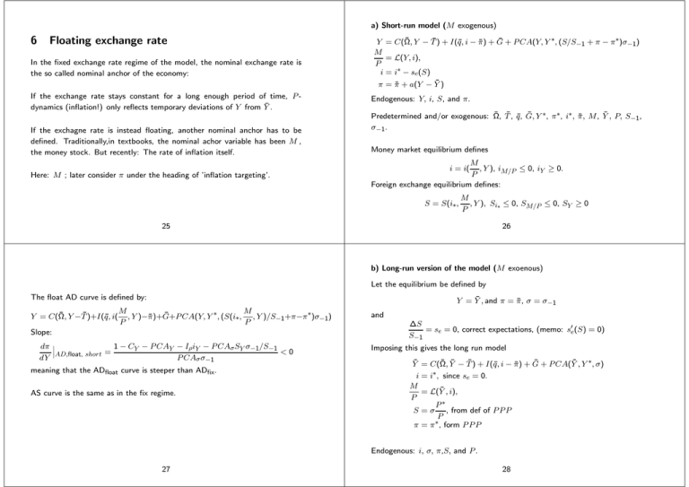
a) Short-run model (M exogenous)
6
Floating exchange rate
In the fixed exchange rate regime of the model, the nominal exchange rate is
the so called nominal anchor of the economy:
If the exchange rate stays constant for a long enough period of time, P dynamics (inflation!) only reflects temporary deviations of Y from Ȳ .
If the exchagne rate is instead floating, another nominal anchor has to be
defined. Traditionally,in textbooks, the nominal achor variable has been M ,
the money stock. But recently: The rate of inflation itself.
Here: M ; later consider π under the heading of ’inflation targeting’.
Y = C(Ω̄, Y − T̄ ) + I(q̄, i − π̄) + Ḡ + P CA(Y, Y ∗, (S/S−1 + π − π ∗)σ−1)
M
= L(Y, i),
P
i = i∗ − se(S)
π = π̄ + a(Y − Ȳ )
Endogenous: Y, i, S, and π.
Predetermined and/or exogenous: Ω̄, T̄ , q̄, Ḡ, Y ∗, π ∗, i∗, π̄, M , Ȳ , P, S−1,
σ−1.
Money market equilibrium defines
M
, Y ), iM/P ≤ 0, iY ≥ 0.
P
Foreign exchange equilibrium defines:
i = i(
S = S(i∗,
M
, Y ), Si∗ ≤ 0, SM/P ≤ 0, SY ≥ 0
P
25
26
b) Long-run version of the model (M exoenous)
Let the equilibrium be defined by
The float AD curve is defined by:
M
M
Y = C(Ω̄, Y −T̄ )+I(q̄, i( , Y )−π̄)+Ḡ+P CA(Y, Y ∗, (S(i∗, , Y )/S−1+π−π ∗)σ−1)
P
P
Slope:
dπ ¯¯
1 − CY − P CAY − IρiY − P CAσ SY σ−1/S−1
<0
¯AD,float, short =
dY
P CAσ σ−1
meaning that the ADfloat curve is steeper than ADfix.
AS curve is the same as in the fix regime.
Y = Ȳ , and π = π̄, σ = σ−1
and
∆S
= se = 0, correct expectations, (memo: s0e(S) = 0)
S−1
Imposing this gives the long run model
Ȳ = C(Ω̄, Ȳ − T̄ ) + I(q̄, i − π̄) + Ḡ + P CA(Ȳ , Y ∗, σ)
i = i∗, since se = 0.
M
= L(Ȳ , i),
P
P∗
S = σ , from def of P P P
P
π = π ∗, form P P P
Endogenous: i, σ, π,S, and P .
27
28
7
Fiscal policy
Predetermined and/or exogenous: Ω̄, T̄ , q̄, Ḡ, Y ∗, M, π ∗, i∗, π̄, Ȳ
More compactly written
Fiscal policy serves several purposes
1. Provision of public goods and services.
Ȳ = C(Ω̄, Ȳ − T̄ ) + I(q̄, i∗ − π̄) + Ḡ + P CA(Ȳ , Y ∗, σ)
M
∗
σ PS
= L(Ȳ , i∗)
2. Redistributive goals. (Equity versus efficiency?)
with σ and S endogenous. Note logically: Since π = π ∗ from P P P , must also
have π̄ = π ∗.
3. Macro-economic stabilization
3. is complementary/alternative to monetary policy, and is our main concern
here
29
30
Fiscal policy in AD-AS model.
Vertical shift in AD curves:
dπ ¯¯
−1
¯AD,f ix,short =
dḠ
P CAσ σ−1
dπ ¯¯
−1
¯AD,float,short =
dḠ
P CAσ σ−1
Hence fiscal policy has larger effect under fixed exchange rate.
Role of capital mobility (optional note)
Baseline model assumes perfect capital mobility. If we (instead) assume imperfect capital mobility we have the following modifications:
1. Only minor in float case. Why? (Money market analysis as before, and
positive relationship between i and S in the foreign exchange marker (same
as the downward sloping “Ei-curve” in the OEM model).
Key mechanism:
In a clean float regime i % in the money market leads to σ % in the market for
foreign exchange. Both effects reduce the effect relative to the fixed exchange
rate regime.
2. In a fixed exchange rate regime, the government might choose to control
money supply, through sterilization. In that case i % also in this regime,
thus reducing the expansive effect.
The conclusion applies to the short-run. In the long run net, exports are
crowded out by increased expenditure in both regimes.
31
32
The activity corrected surplus
The budget surplus
Replace the baseline model’s assumption about exogenous taxes T̄ , with a
tax-function
While the rationale for modern fiscal policy is to affect the overall activity level
(and thus unemployment rates), it most direct impact is on the government’s
own financial situation.
That side of the issue is always important, i.e., prudent governments always try
to keep down/revert deficits in order to maintain financial independence (for a
rainy day, and in order to maintain and strengthen the beliefs in the stability
of the currency and the solvency of the government).
Sometimes, government deficients become the overriding concern of financial
policy, either because of past sins (large debt), or because of new political
priorities.
T = τY
which (though exceedingly simple) is more realistic. Clearly the tax-function
makes the government primary surplus
T −G
dependent on whether the activity level is high or low.
Today a good deal of emphasis on activity correction, which would be
τ Ȳ − G
A much used decomposition of the budget is then
τ (Y − Ȳ ) + τ Ȳ − G
33
34
Debt financing and debt stabilization
In practice (more complicated computation though).
Used to characterize a budget as “really” expansionary or contractive. Popular
among politicians.
Using B&W notation, the change in real public debt (B), is equal to the total
budget deficit
∆B = G − T + rB
(15.1)
where r is a real interest rate. rB is referred to as “debt service”.
Alternative to using model multipliers of Y wrt G to characterize the budget.
Seemingly more free of assumption, but in reality just as model dependent (cf
calculating the trend GDP output level Y ).
Over time governments must stabilize the debt to income ratio B/Y
B
G − T + rB
∆( ) =
Y
Y
Rewrite left hand side
B
∆B ∆Y
∆BY − ∆Y B
∆ =
=
−
B
2
Y
Y
Y
Y
so that (*) can be written
B
B
∆( ) = G − T + (r − g)
Y
Y
35
36
(*)
(15.3)
To stabilize debt at a certain level, the primary surplus T − G must equal
B . “Easiest” when interest rates are low and growth is high (e.g.,
(r − g) Y
Europe in the 1950’s and 1960s).
Deficit reduction has been the way chosen by many European countries as a
result of the Maastricht treaty in 1991 and the Stability and Growth Pact of
1997. Has contributed to high European unemployment, though only temporary according to AD-AS with Phillips curve.
Modifications: Seigniorage and inflation tax.
Down the years governments debt (in real terms!) has also been able to reduced
by high inflation, which (as we have seen) takes away the gains from owing
fixed income assets (bonds), hence is referred to as inflation tax.
Adoption of low inflation as a target of monetary policy as greatly reduced the
inflation tax.
In practice, not all public debt is interest bearing. If the government finances a
deficit by printing money, it obtains an interest free loan from the public. This
source of “income” to the central government is called seigniorage. Without
the monopoly right to printing money the government would have sell bonds
and pay interest instead.
The Stability pact “forbids” this form of debt financing.
38
37
Issues in demand management.
Slope of AS schedule and adjustment lags
The rationale and scope for “activist fiscal policy” is a main controversy in
economics.
B&W point out that the rationale for demand adjustment is larger if short-run
AS curve is flat and it takes (long) time before the short sun curve “moves
back” to the vertical long run position.
B&W ch 16 is highly recommended.
Here, comment only on a few of the issues covered by B&W:
Answer hinges on the shape of the Phillips curve (non-linearities is essential),
and about how fast
1. Slope of AS schedule and adjustment lag
• core inflation adjusts
2. Policy and effectiveness lags
• and also how fast unemployment changes (not mentioned by B&W) towards its natural rate
3. Lucas critique
However, a more overriding concern is the status of the Phillips curve natural
rate model itself.
39
40
Policy and effectiveness lags
Is the long run AS curve vertical?
As we have seen there are competing models of wage and price setting which
refute that thesis.
Aukrust/bargaining model: Inflation stabilizes at the foreign rate of inflation
at “any” level of unemployment. Implying that the equilibrium level of unemployment need not coincide with the Phillips curve natural rate.
A very relevant caution against too ambitious demand control is related to the
fact that various lags makes it difficult in practice to carry out the intention of
counter cyclical fiscal policy.
1. Recognition lag (data measurement)
2. Decisions lag (political system)
3. Implementation lag (“red tape”)
4. Effectiveness lag (from change in instrument to effect in target)
42
41
8
Lucas critique
No controversy that expectations are important in macroeconomics.
The Lucas critique takes the extreme view that expectations are rational and
that they dominate the economic decisions of households and firms. Hence
impossible to predict reactions to economic policy changes on the basis of
current and past behaviour (e.g., as summarized in an econometric consumption
function).
If valid empirically, the Lucas critique takes away the rationale for demand
management.
Supply-Side Policy (B&W ch 17)
The important sections for our course is section 17.4.
Note in particular the discussion about active and passive labour market programmes, Box. 17.5., which reflects the view that the comparatively low Nordic
unemployment rates is due to active programmes.
Rødseth and Nymoen (2003) find no strong evidence for the positive influence
of programmes on employment, and at the same time report that demand
management and devaluations have been important.
Role of labour unions.
However, empirical tests show that the empirical relevance of the Lucas critique
is overstated.
Separate handout provides shows that if bargaining is coordinated (“centralized”), union based wage setting might entail quite flexible wages (in line with
Gjedrem’s talk at the start of the term).
43
44