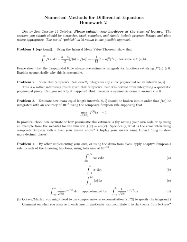
Numerical Methods for Differential Equations
Homework 2
Due by 2pm Tuesday 13 October. Please submit your hardcopy at the start of lecture. The
answers you submit should be attractive, brief, complete, and should include program listings and plots
where appropriate. The use of “publish” in Matlab is one possible approach.
Problem 1 (optional). Using the Integral Mean Value Theorem, show that
Z
b
f (x) dx −
a
b−a
1
[f (b) + f (a)] = − (b − a)3 f 00 (η) for some η ∈ (a, b).
2
12
Hence show that the Trapezoidal Rule always overestimates integrals for functions satisfying f 00 (x) ≥ 0.
Explain geometrically why this is reasonable.
Problem 2. Show that Simpson’s Rule exactly integrates any cubic polynomial on an interval [a, b].
This is a rather interesting result given that Simpson’s Rule was derived from integrating a quadratic
polynomial proxy. Can you see why it happens? Hint: consider a symmetric domain around x = 0.
Problem 3. Estimate how many equal length intervals [0, 2] should be broken into in order that f (x) be
integrated with an accuracy of 10−5 using the composite Simpson rule supposing that
max |f (4) (x)| = 1.
x∈[0,2]
In practice, check how accurate or how pessimistic this estimate is (by writing your own code or by using
an example from the website) for the function f (x) = cos(x). Specifically, what is the error when using
composite Simpson with n from your answer above? (Display your answer using format long to show
more decimal places).
Problem 4. By other implementing your own, or using the demo from class, apply adaptive Simpson’s
rule to each of the following functions, using tolerance of 10−10 .
π/2
Z
cos x dx
(a)
|x| dx,
(b)
0
Z
1
−1
Z
3/2
|x| dx
(c)
−1
Z
∞
−∞
1
2
√ e−x /2 dx
2π
Z
5
approximated by
−5
1
2
√ e−x /2 dx
2π
(d)
(In Octave/Matlab, you might need to use component-wise exponentiation (x.^2) to specify the integrand.)
Comment on what you observe in each case; in particular, can you relate it to the theory from lectures?
Problem 5.
1. Consider the “1 -2 1” rule for computing the second deriviative from lectures. Taking u(x) = esin(x)
and x = 3, compute the error for h = 0.1 and h = 0.05.
2. In lecture, we mentioned that this rule would eventually fail for small enough h. Design a study for
various h’s to find the minimum value of h below which the error begins to increase. Hint: make a
log-log plot, label your point as hmin . What is the slope of the line for h > hmin ?
3. Does this result change much if you use a different smooth function for f ?
4. Determine hmin when using single precision arithmetic (i.e., repeat the experiment wholly in single
precision arithmetic—“help single” on Octave/Matlab, “whos” is very helpful)
5. Determine hmin for the forward difference approximation for ux .
6. Determine hmin for the centered difference approximation for ux .
7. Strictly optionally: if you are working in an appropriate computing environment (probably Fortran
or C) then try with extended precision or quadruple precision.