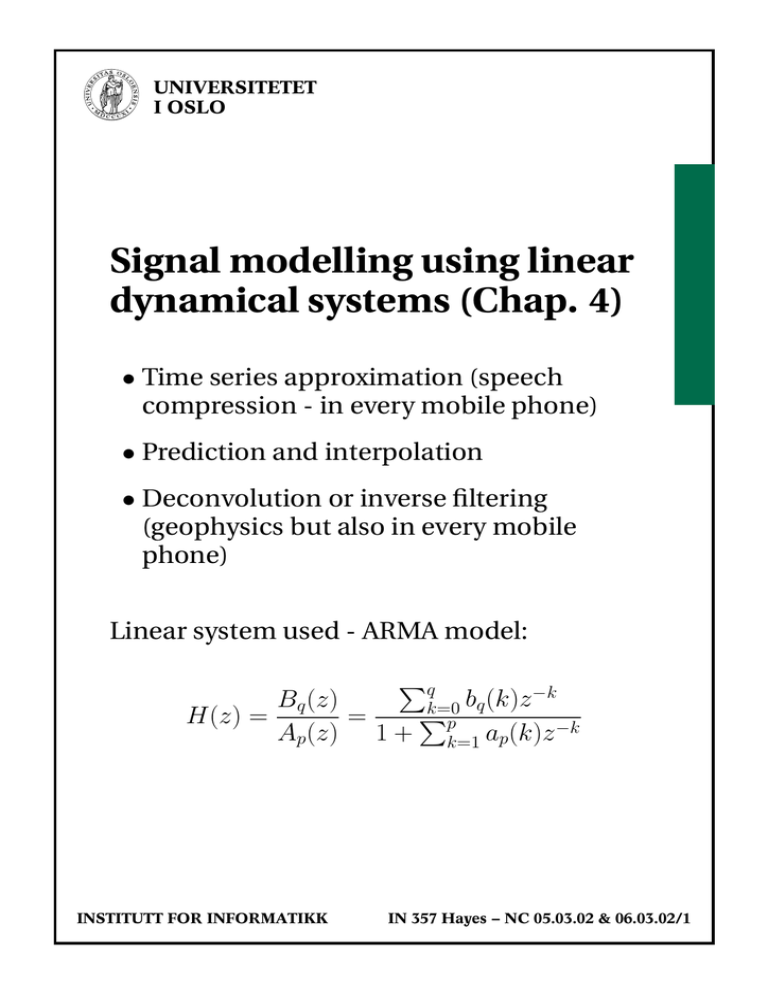
UNIVERSITETET
I OSLO
Signal modelling using linear
dynamical systems (Chap. 4)
• Time series approximation (speech
compression - in every mobile phone)
• Prediction and interpolation
• Deconvolution or inverse filtering
(geophysics but also in every mobile
phone)
Linear system used - ARMA model:
Pq
−k
b
(k)z
Bq (z)
q
k=0
P
=
H(z) =
Ap(z) 1 + pk=1 ap(k)z −k
INSTITUTT FOR INFORMATIKK
IN 357 Hayes − NC 05.03.02 & 06.03.02/1
UNIVERSITETET
I OSLO
First problem - Approximate a given time
series x(n), n = 0, 1, · · · by the impulse response
h(n) of the system H(z). We have:
h(n) +
p
X
ap(k)h(n − k) = bq (n)
k=1
h(n), bq (n) = 0, n < 0 and bq (n) = 0, n > q
Given e0(n) = x(n) − h(n), find
ap(k), k = 1, · · · , p and bq (k), k = 0, · · · , q to
minimize
ELS =
∞
X
|e0(n)|2
n=0
Leads to non-linear problem in ap(k) and bq (k)
(p. 132 - 133).
Three linear suboptimal solutions
considered: Padé, Prony, and Shank.
INSTITUTT FOR INFORMATIKK
IN 357 Hayes − NC 05.03.02 & 06.03.02/2
UNIVERSITETET
I OSLO
Note:
• h(n) is the solution of a linear difference
equation ⇒ approximation basically
constrained to sum of (complex)
exponential sequences
• Selection of model order (p and q) not
treated in any detail
• Statistical properties of estimators not
considered
Main idea behind suboptimal methods:
Assume that x(n) (approximately) is the
impulse response of a linear system. Then
there must be a structure (more or less) given
by:
x(n) +
p
X
ap(k)x(n − k) = bq (n), x(n) = 0, n < 0
k=1
for some ap(k), k = 1, · · · , p and
bq (n), n = 0, · · · , q
INSTITUTT FOR INFORMATIKK
IN 357 Hayes − NC 05.03.02 & 06.03.02/3
UNIVERSITETET
I OSLO
Padé: Seeks an exact fit to a difference
equation for n = 0, · · · , p + q
1. Fix p, q
2. Determine ap(k), k = 1, · · · , p from the
constraint
x(n)+
p
X
ap(k)x(n−k) = 0, n = q+1, · · · , q+p
k=1
This gives p linear equations with p
unknowns. Go to 1. if equations are poorly
conditioned (p should be reduced).
3. With ap(k) given, determine
bq (n), n = 0, · · · , q from
bq (n) = x(n) +
p
X
ap(k)x(n − k)
k=1
4. Check fit for n > q + p and possibly go to 1.
INSTITUTT FOR INFORMATIKK
IN 357 Hayes − NC 05.03.02 & 06.03.02/4
UNIVERSITETET
I OSLO
Prony: Seeks an exact fit to a difference
equation for n = 0, · · · , q and a least squares
fit for n > q.
1. Fix p, q
2. Determine ap(k), k = 1, · · · , p by
minimizing
Ep,q =
∞
X
(e(n))2, e(n) = x(n)+
n=q+1
p
X
ap(k)x(n−k)
k=1
Gives a linear least squares problem in
ap(k). Go to 1. if equations are poorly
conditioned (p should be reduced).
3. With ap(k) given, determine
bq (n), n = 0, · · · , q as for Padé
bq (n) = x(n) +
p
X
ap(k)x(n − k)
k=1
4. Check min. Ep,q (Hayes eq. 4.44) and
possibly go to 1.
INSTITUTT FOR INFORMATIKK
IN 357 Hayes − NC 05.03.02 & 06.03.02/5
UNIVERSITETET
I OSLO
Shanks: Performs a least squares fit to a
difference equation for n > 0 but in two steps
1. Fix p, q
2. Determine ap(k), k = 1, · · · , p as for Prony,
i.e. by a least squares fit over n > q
3. With ap(k) given, determine
bq (n), n = 0, · · · , q by (Fig. 4.11)
(a) Compute the impulse response g(n) for
1
Ap (z) , i.e.
g(n) +
p
X
k=1
(b) Minimize Es =
where
ap(k)g(n − k) = δ(n)
P∞
0
2
n=0 (e (n))
e0(n) = x(n)− x̂(n) = x(n)−
w.r.t. bq
q
X
bq (l)g(n−l)
l=0
4. Check min. Es (Hayes eq. 4.67) and
possibly go to 1.
INSTITUTT FOR INFORMATIKK
IN 357 Hayes − NC 05.03.02 & 06.03.02/6