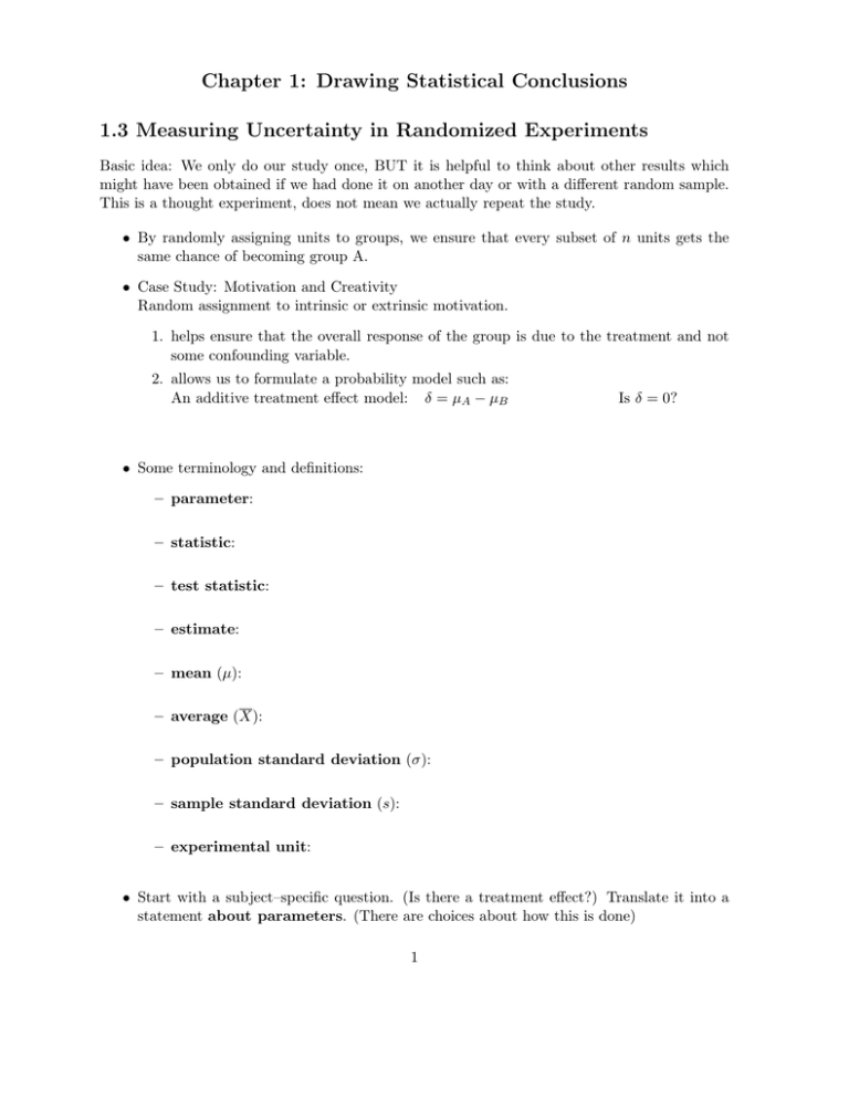
Chapter 1: Drawing Statistical Conclusions
1.3 Measuring Uncertainty in Randomized Experiments
Basic idea: We only do our study once, BUT it is helpful to think about other results which
might have been obtained if we had done it on another day or with a different random sample.
This is a thought experiment, does not mean we actually repeat the study.
• By randomly assigning units to groups, we ensure that every subset of n units gets the
same chance of becoming group A.
• Case Study: Motivation and Creativity
Random assignment to intrinsic or extrinsic motivation.
1. helps ensure that the overall response of the group is due to the treatment and not
some confounding variable.
2. allows us to formulate a probability model such as:
An additive treatment effect model: δ = µA − µB
Is δ = 0?
• Some terminology and definitions:
– parameter:
– statistic:
– test statistic:
– estimate:
– mean (µ):
– average (X):
– population standard deviation (σ):
– sample standard deviation (s):
– experimental unit:
• Start with a subject–specific question. (Is there a treatment effect?) Translate it into a
statement about parameters. (There are choices about how this is done)
1
– Null Hypotheses: No treatment effect
– Alternative Hypotheses: Some treatment effect
– For the additive treatment effects model, we focus on a shift in means, δ = µA − µB
H0 :
Ha :
– A test statistic is used to measure the consistency of the null hypothesis and the data.
– For reference: how much does the test stat vary under different random allocations of
treatment given H0 is true? Is the one test stat we have observed unusual compared
to all those we might have seen?
– Randomization distribution of the test statistic: All test statistic values for every
possible outcome of randomly assigning the units to groups.
∗ In small (toy) examples as on HW1, we can look at all possible randomizations.
∗ With moderate sample sizes, the number of possible randomizations is too large
to handle, so we can just randomly look at 1000 or so of them (See Displays 1.7
and 1.8).
– Randomization test is based on the premise: there is no real difference between the
treatments (H0 , no effect on the mean), so all that’s going on is random selection into
groups A and B. Group means will naturally vary, so we don’t expect the difference
to be zero. All possible randomizations shows us what to expect when H0 is true..
– What is a p-value in the context of a randomized experiment?
– Ways to obtain a p-value:
1. EXACT: Find all possible regroupings of the data (create the randomization
distribution) and find the proportion of these that produce a test statistic as
extreme or more extreme than the observed one.
2. APPROXIMATE the randomization distribution by simulating a large number of
randomizations and finding the proportion of these that produce a test statistic
as extreme or more extreme than the observed one.
3. MOST COMMON: Approximate the randomization distribution with a mathematical curve based on assumptions about the distribution of the response and
the form of the test statistic. Often the normal or t distributions.
1.4 Measuring Uncertainty in Observational Studies
• In an observational study, there is no random group assignment. Instead, we observe
covariates.
2
• There is a chance mechanism for sample selection if we sample at random. This provides a probability model connecting the distribution of the test statistic to the chance
mechanism.
• IDEA: Visualize hypothetical replications of a study under different randomly selected samples.
1.4.1 A probability model for random sampling
• Randomly select units from one or more populations.
• For comparing two populations:
1. Select n1 units from population 1 such that all subsets of size n1 have the same chance
of selection.
2. Select n2 units in the same manner from population 2 independent of those from
population 1. (the sample drawn from population 1 should not influence how the
sample from population 2 is drawn.)
• Ask, “Do the population means differ?”
– Is the observed difference between the sample averages real or just a fluke from random
sampling?
– Rewrite the question in terms of parameters of a model:
– Estimate the parameter of interest (i.e. what statistic should we use?).
– A sampling distribution for (Y 1 − Y 2 ) is represented by a histogram of all values for
the statistic from all possible samples that can be drawn from the two populations.
∗ How does this differ from the randomization distribution we discussed in the
previous section?
∗ All confidence intervals and p-values are based on our knowledge of the sampling
distribution.
1.4.2 A permutation distribution
• Example: The sex discrimination case study.
– Is it an experiment or observational study?
3
– Were people selected via random sampling?
– Based on our answers where does a chance mechanism come into the picture? (It’s a
stretch.)
– Inference is based on a fictitious (pretend) probability model. Pretend that the employer assigned the set of starting salaries to employees at random (that’s easier than
changing genders at random). We then compare the observed salary difference between males and females to what we would expect if the salaries were handed out at
random. We still only see one difference in means. The others are imagined under
the probability model.
∗ Null Hypothesis: no difference between males and females, except that some
people got lucky and others didn’t.
∗ Imagine repeating the process when the null is true. Redistribute salaries at
random to each person.
∗ Permutation distribution: how does the statistic Y 1 − Y 2 change under different randomizations when only chance is operating?
∗ The p-value is the proportion of statistics as extreme or more extreme (farther
from 0) than the one we observed.
∗ How is a permutation distribution different from a randomization distribution?
∗ What is the proper scope of inference for the sex discrimination case study?
1.5.1 Graphical Methods
You are responsible for understanding and being able to produce the following graphs:
• Histograms
• Stem-and-Leaf Diagrams
• Box plots
• Scatter plots
Rcode:
4
fishDiet <- c( 8,12,10,14,2,0,0)
regDiet <- c(-6,0,1,2,-3,-4,2)
stem(fishDiet)
stem(regDiet) ## hard to compare
boxplot(fishDiet, regDiet, xlab = "Diet")
mtext(side=1, at = 1:2, c("Fish Oil","Regular Oil"))
## make a data table
diets <- data.frame( deltaDBP = c(fishDiet,regDiet), type = rep(c("fish","regular"),each=7))
boxplot(deltaDBP ~ type, data = diets, ylab="Change in DBP")
hist(fishDiet)
hist(regDiet)
require(lattice) ## load fancier plotting package
histogram(~deltaDBP|type,diets) ## works only after lattice is loaded
height <- c(68.4, 68.2, 72.7, 71.4, 74.0, 76.2, 74.4, 71.2, 71.7, 67.4, 73.0, 64.3)
earnings <- c(60.8, 54.4, 69.2, 59.9, 69.3, 77.1, 73.8, 68.2, 63.8, 49.4, 67.1, 44.7)
plot(x=height, y=earnings)
1.5.5 On Being Representative
• Random samples and randomized experiments are representative in the same sense that
flipping a coin is fair.
• Examination of the results of randomization or random sampling can usually expose ways
in which the chosen sample is not representative. However, do not abandon the procedure when the result is suspect.
– Uncertainty about representativeness is incorporated into the statistical analysis itself.
If you abandon randomization (or mess with it) than there is no way to accurately
express uncertainty.
Chapter 1 overview questions:
1. What is the main reason that cause-and-effect relationships cannot be inferred from observational studies?
2. Why does randomization allow cause-and-effect statements to be made?
Work through the conceptual questions (1 through 12) in the book’s section 1.7.
5