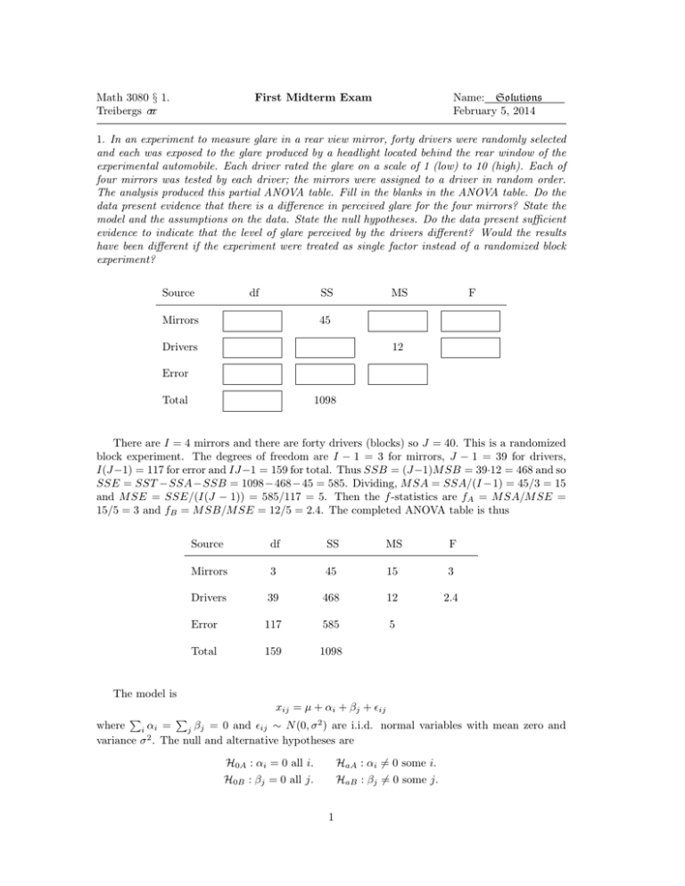
Math 3080 § 1.
Treibergs σ−
ιι
First Midterm Exam
Name: Solutions
February 5, 2014
1. In an experiment to measure glare in a rear view mirror, forty drivers were randomly selected
and each was exposed to the glare produced by a headlight located behind the rear window of the
experimental automobile. Each driver rated the glare on a scale of 1 (low) to 10 (high). Each of
four mirrors was tested by each driver; the mirrors were assigned to a driver in random order.
The analysis produced this partial ANOVA table. Fill in the blanks in the ANOVA table. Do the
data present evidence that there is a difference in perceived glare for the four mirrors? State the
model and the assumptions on the data. State the null hypotheses. Do the data present sufficient
evidence to indicate that the level of glare perceived by the drivers different? Would the results
have been different if the experiment were treated as single factor instead of a randomized block
experiment?
Source
df
SS
Mirrors
MS
F
45
Drivers
12
Error
Total
1098
There are I = 4 mirrors and there are forty drivers (blocks) so J = 40. This is a randomized
block experiment. The degrees of freedom are I − 1 = 3 for mirrors, J − 1 = 39 for drivers,
I(J−1) = 117 for error and IJ−1 = 159 for total. Thus SSB = (J−1)M SB = 39·12 = 468 and so
SSE = SST −SSA−SSB = 1098−468−45 = 585. Dividing, M SA = SSA/(I −1) = 45/3 = 15
and M SE = SSE/(I(J − 1)) = 585/117 = 5. Then the f -statistics are fA = M SA/M SE =
15/5 = 3 and fB = M SB/M SE = 12/5 = 2.4. The completed ANOVA table is thus
Source
df
SS
MS
F
Mirrors
3
45
15
3
Drivers
39
468
12
2.4
Error
117
585
5
Total
159
1098
The model is
xij = µ + αi + βj + ij
where i αi = j βj = 0 and ij ∼ N (0, σ 2 ) are i.i.d. normal variables with mean zero and
variance σ 2 . The null and alternative hypotheses are
P
P
H0A : αi = 0 all i.
HaA : αi 6= 0 some i.
H0B : βj = 0 all j.
HaB : βj 6= 0 some j.
1
To test if the means are significantly different due to mirrors, see if the corresponding f value
exceeds the critical f.05,3,117 ≈ f.05,3,100 = 2.70, which is the more conservative nearby number in
Table A9. Thus fA = 3 > 2.70 so there are a significant difference in glare rating due to mirrors.
If there had been no blocking, extra variability would have come from drivers and the corresponding M SE 0 would have been larger and the fA0 would have been smaller. Indeed, there
would have been no sum square subtracted for blocking and SSE 0 = SSE + SSB = 953,
dfE = 117+39 = 156 and M SE 0 = 953/156 = 6.11 so fA0 = M SA/M SE 0 = 12/6.11 = 1.96. Now
the critical f.05,3,156 ≈ 2.70 and the differences due to mirrors would not have been significant.
c InsectSprays, 6 different insecticides were applied to agricul2. In a canned data set from R,
tural experimental units. 12 samples of each type were tested. Counts of insects surviving were
reported. The data is analyzed as a single factor fixed effects model. The data indicate that there
are significant differences in counts due to sprays. Use Tukey’s procedure to identify differences in
the true average insect counts among the six sprays. Use the method of underscoring to illustrate
your conclusions. Write a sentence summarizing your results.
> a1 = aov(count ~ spray); summary(a1)
Df Sum Sq Mean Sq F value
Pr(>F)
spray
5 2668.8 533.77 34.702 < 2.2e-16 ***
Residuals
66 1015.2
15.38
--Signif. codes: 0 *** 0.001 ** 0.01 * 0.05 . 0.1
1
> tapply(count, spray, mean)
A
B
C
14.500000 15.333333 2.083333
D
4.916667
E
F
3.500000 16.666667
The model is xij = µi + ij where ij ∼ N (0, σ 2 ) are i.i.d. normal. The simultaneous Tukey
CI’s for differences in all pairs of I = 6 means, µi − µj are given by
r
M SE
X i· − X j· ± q(α, I, I(J − 1))
J
where the studentized range q(.05,
Table A10. It follows that if the differences
p6, 66) ≈ 4.16 from p
are not significant if |µi − µj | < q M SE/J = 4.16 ∗ 15.38/12 = 4.71. We sort the means from
smallest to largest.
C
E
D
2.083333
3.500000
4.916667
--------------------------------
A
B
F
14.500000
15.333333
16.666667
---------------------------------
Then we see that |µC − µE |, |µC − µD |, |µE − µD |, |µA − µB |, |µA − µC | and |µB − µC | are less
than 4.71 but all other pairs are greater. The resulting underscoring pattern has two groups of
means that are not significantly different. We may summarize the result as follows: The counts
for sprays C, D and E are not significantly different from one another; the counts for sprays A,
B and F are not significantly different from one another; but the counts for any pair one from the
first group and the other from the second group differ significantly.
2
3. Suppose that in a one factor fixed effects model
where i.i.d. ij ∼ N (0, σ 2 )
xij = µi + ij
three different treatments are measured with two samples per treatment. If we observe
Treatment
1
2
xi
1
19
15
17
2
16
20
18
3
29
21
25
Define what an effect αi is in general. What is the estimator of α
c3 from this data? What is a
residual? What is the residual r3,1 for this data? What is SSA for this data? What is M SE for
this data?
An effect is the difference of the population
mean in the presence of a factor and the grand
P
population mean. If we put µ = I1 i µi then the effect αi = µi − µ. An estimator is αbi =
P
µbi − µ̂ = X i· = X ·· so in this case α
c3 = x3· − x·· = 25 − 20 = 5 where X i· = J1 j Xij and so
P
here x·· = I1 i xi· = 13 (17 + 18 + 25) = 20.
The residual is the difference between the observed and the fitted value. In this case, Rij =
d
Xij − X
ij . In particular here r3,1 = x3,1 − x3,1 = 29 − 25 = 4 .
By definition,
I X
J
X
SSA =
(X i · −X ·· )2
i=1 j=1
so here
SSA = 2 (17 − 20)2 + (18 − 20)2 + (25 − 20)2 = 2(9 + 4 + 25) = 76 .
By definition,
I
M SE =
1X 2
S
I i=1 i
so here
M SE =
1
3
1
1
(19 − 17)2 + (15 − 17)2 +
(16 − 18)2 + (20 − 18)2
2−1
2−1
1
1
+
(29 − 25)2 + (21 − 25)2
= (8 + 8 + 32) = 16 .
2−1
3
Other formulas may also be used. But as always, to show that the correct procedure is being
used, it is important to write the formula before plugging values.
3
4. Artificial joints were studied in an article by Macdonald et al in Proceedings of the Institution
of Mechanical Engineers, 2000. They compared two materials and three taper neck lengths. Five
measurements of friction were made for each combination of material and neck length. State the
model and the assumptions on the data. State the null hypotheses. From the ANOVA table, what
conclusions do you draw? For each of the six diagnostic plots for this data on the next page, state
what the plot says the data or about how well the data satisfies the hypotheses.
Taper Material
CPTi-ZrO2
CPTi-ZrO2
CPTi-ZrO2
TiAlloy
TiAlloy
TiAlloy
Neck Length
Short
Medium
Long
Short
Medium
Long
Coefficient of Friction
0.254 0.220 0.320 0.175
0.195 0.185 0.296 0.131
0.281 0.259 0.178 0.180
0.289 0.197 0.150 0.184
0.220 0.329 0.118 0.154
0.196 0.481 0.158 0.156
> a1=aov(y ~ Material * Neck); summary(a1)
Df
Sum Sq Mean Sq F value
Pr(>F)
Material
1 0.059052 0.059052 23.6304 5.913e-05 ***
Neck
2 0.028408 0.014204 5.6840 0.009533 **
Material:Neck 2 0.009089 0.004544 1.8185 0.183924
Residuals
24 0.059976 0.002499
4
0.177
0.178
0.198
0.201
0.199
0.210
The model is a two factor fixed effects model with replication. There are I = 2 materials,
J = 3 neck lengths and K = 5 replicates per cell. The model is
xijk = µ + αi + βj + γij + ijk
where the sum over any one index for αi , βj and γij is zero and ijk ∼ N (0, σ 2 ) are i.i.d. normal
variables. The null and alternative hypotheses are
H0A : αi = 0 all i.
HaA : αi 6= 0 some i.
H0B : βj = 0 all j.
HaB : βj 6= 0 some j
H0AB : γij = 0 all i, j.
HaAB : γij 6= 0 some i, j.
From the ANOVA table, the interactions have large p-value so H0AB cannot be rejected and so
the interactions are plausibly zero. On the other hand the p-values for neck and material are small
so both H0A and H0B are rejected. Both have significant effects on the coefficient of friction.
The various diagnostic plots give informatin about the data and how well the data satisfies
the assumptions.
1. Observed vs. Fitted. Plot shows that the the variation seems to increase with fitted value,
so that there may be doubt on equality of variance for each cell.
2. Boxplot. The means are slightly different for different neck sizes. We also see that the
spread varies for different levels of the factor neck so that there may be doubt on equality
of variance for each neck size.
3. Design Plot. Shows mean friction for different levels of the two factors. Both neck and
material means vary with factor levels.
4. Observed vs. Factors. Gives a dot plot for every factor combination. Not only are the
centers dependent on factor combinations but the two materials seem to have different
spreads showing the equality of variance for each cell may be in doubt.
5. Standardized Residuals vs. Fitted. This time the observations are centered and divided
by the grand standard deviation. Still see the horn pattern: the variability increases with
fitted value putting doubt on the equality of variance.
6. QQ Normal Plot of Standardized Residuals. This one has a pronounced “N” shape indicating heavy tails for the residuals. This is another indicator that the epsilons may not be
normally distributed.
5
5. PVC is made by polymerizing a vinyl chloride monomer in a batch chemical reactor where
it is mixed with water to produce a resin of desired molecular weight. A 1998 study in Quality
Engineeringmeasured the effect of operators and resin railcars on the particle size of the resin.
The operators and railcars were both randomly selected from their respective populations because
the objective of the study was to measure the variation due to operators and due to railcars. Two
resin samples were selected from each operator-railcar combination. Is this a fixed effects, random
effects or mixed model? State the model and the assumptions on the data. Is there an interaction
due to operator and railcar? State the null and alternative hypotheses. State the test statistic.
What is your conclusion? What can you conclude about the effect of railcar on particle size?
State the null and alternative hypothesis, the test statistic, the level 0.05 rejection region and your
conclusion.
> a1=aov(size ~ Operator * Railcar); summary(a1)
Df Sum Sq Mean Sq F value
Pr(>F)
Operator
2 20.902 10.451 7.1776 0.003603 **
Railcar
7 283.871 40.553 27.8516 4.845e-10 ***
Operator:Railcar 14 14.142
1.010 0.6937 0.758885
Residuals
24 34.945
1.456
This is a random effects model. We assume
xijk = µ + Ai + Bj + Cij + ijk
where all the random variables Ai , Bj Cij and ijk are independent RV’s that satisfy
2
Ai ∼ N (0, σA
),
2
Bj ∼ N (0, σB
),
2
Cij ∼ N (0, σC
),
ijk ∼ N (0, σ 2 ).
The null and alternative hypotheses are
2
H0A : σA
= 0.
2
HaA : σA
6= 0.
2
H0B : σB
= 0.
2
HaB : σA
6= 0.
2
H0AB : σC
= 0.
2
HaAB : σC
6= 0.
To test for variability due to interaction of the two factors, the statistic is fAB = M SAB/M SE =
2
is
0.6937 which has a p-value 0.758885. Thus we cannot reject H0AB and conclude that σC
plausibly zero: there is no significant variability of particle size due to interaction.
To test for variability due to railcar, the statistic is fB = M SB/M SAB = 40.553/1.010 =
40.151. We reject H0B if fB exceeds the critical value f (0.05, 7, 14) = 2.76 from table A9. Thus
2
we reject H0B and conclude that σB
is significantly nonzero: there is variability on particle size
due to railcars.
6