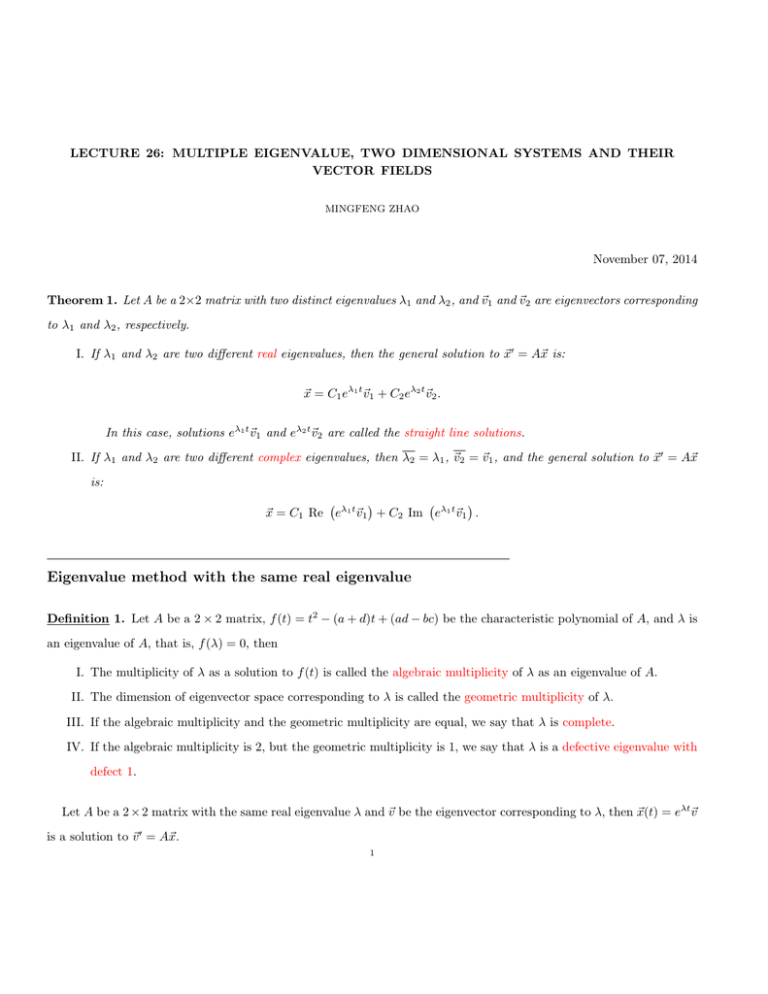
LECTURE 26: MULTIPLE EIGENVALUE, TWO DIMENSIONAL SYSTEMS AND THEIR
VECTOR FIELDS
MINGFENG ZHAO
November 07, 2014
Theorem 1. Let A be a 2×2 matrix with two distinct eigenvalues λ1 and λ2 , and ~v1 and ~v2 are eigenvectors corresponding
to λ1 and λ2 , respectively.
I. If λ1 and λ2 are two different real eigenvalues, then the general solution to ~x0 = A~x is:
~x = C1 eλ1 t~v1 + C2 eλ2 t~v2 .
In this case, solutions eλ1 t~v1 and eλ2 t~v2 are called the straight line solutions.
II. If λ1 and λ2 are two different complex eigenvalues, then λ2 = λ1 , ~v2 = ~v1 , and the general solution to ~x0 = A~x
is:
~x = C1 Re eλ1 t~v1 + C2 Im eλ1 t~v1 .
Eigenvalue method with the same real eigenvalue
Definition 1. Let A be a 2 × 2 matrix, f (t) = t2 − (a + d)t + (ad − bc) be the characteristic polynomial of A, and λ is
an eigenvalue of A, that is, f (λ) = 0, then
I. The multiplicity of λ as a solution to f (t) is called the algebraic multiplicity of λ as an eigenvalue of A.
II. The dimension of eigenvector space corresponding to λ is called the geometric multiplicity of λ.
III. If the algebraic multiplicity and the geometric multiplicity are equal, we say that λ is complete.
IV. If the algebraic multiplicity is 2, but the geometric multiplicity is 1, we say that λ is a defective eigenvalue with
defect 1.
Let A be a 2 × 2 matrix with the same real eigenvalue λ and ~v be the eigenvector corresponding to λ, then ~x(t) = eλt~v
is a solution to ~v 0 = A~x.
1
2
MINGFENG ZHAO
I. If λI2 − A = 0, that is, λ is a geometric eigenvalue, then the general solution to ~x0 = A~x is


 
1
0
 + eλt   .
~x(t) = eλt 
0
1
II. If λI2 − A 6= 0, that is, λ is a defective eigenvalue, then another linearly independent solution ~y to ~x0 = A~x has
the form ~y (t) = eλt (t~v + w)
~ for some vector w
~ to be determined. After a simple computation, we will know that
w
~ satisfies
(λI2 − A)w
~ = −~v .

Example 1. Solve ~x0 = 

2
0
2
0
0
2

 ~x.

, it’s easy to say that A has only one eigenvalue λ = 2 and 2I2 − A = 0, that is, λ = 2 is a geometric
0 2
eigenvalue of A. So the general solution to ~x0 = A~x is:
Let A = 

2t
~x(t) = C1 e 
1


2t
 + C2 e 
0
det (λI2 − A) = det 
.
1

 x0 = 3x1 + x2
1
Example 2. Find the general solution to
.
 x0 = 3x
2
2


0
 x = 3x1 + x2
3
1
The coefficient matrix of the system
is A = 
 x0 = 3x
0
2
2


0
λ−3
−1
0
λ−3
1

. First, let’s find eigenvalues of A, then
3

 = (λ − 3)2 = 0.
Then λ1 = λ2 = 3. Now let’s solve


3
1
0
3
0
−1
0
0

x1



 = 3
x2
x1

.
x2
Then



So 
x1
x2


 = x1 
1
0


x1

x2


=
0

.
0

. Hence we know that λ = 3 is the only one eigenvalue for A, ~v = 
1

 is the eigenvector,
0
and 3I2 − A 6= 0, that is, λ = 3 is a defective eigenvalue of A. Then ~y (t) = e3t~v is a solution to ~x0 = A~x.
LECTURE 26: MULTIPLE EIGENVALUE, TWO DIMENSIONAL SYSTEMS AND THEIR VECTOR FIELDS
3
Let ~x = e3t (t~v + w)
~ = t~y (t) + e3t w
~ be another linearly independent solution to ~x0 = A~x, then
~x0 = ~y (t) + t~y 0 (t) + 3e3t w
~ = A(t~y (t) + e3t w)
~ = tA~y (t) + e3t Aw.
~
Since ~y (t) is a solution to ~x0 = A~x, then
~y (t) + 3e3t w
~ = e3t Aw.
~
Since ~y (t) = e3t~v , then e3t~v + 3e3t w
~ = e3t Aw,
~ that is, ~v + 3w
~ = Aw.
~ Hence, (3I2 − A)w
~ = −~v , that is,


 

0 −1
w
−1

 1  = 

0 0
w2
0

So we can take w1 = 0 and w2 = 1, that is, w
~ =

0
. So another solution is
−1
 
e3t (t~v + w)
~ = e3t t 
1


+
0
0


 = e3t 
1
t

.
1
Therefore, the genera solution to ~x0 = A~x is:

~x = C1 e3t 
1


 + C2 e3t 
0
t


=
1
C1 e3t + C2 te3t
C2 e3t

.
Two dimensional systems and their vector fields
To draw the vector field of a general system ~x0 = f~(t, ~x):
I. Plot the tx1 x2 -space.
II. Select points as many as possible in the plane, say P1 , P2 , · · · , Pn .
III. At each point Pi , draw a short arrow with direction (1, f1 (Pi ), f2 (Pi )).
Remark 1. For any given initial data ~x(t0 ) = P0 , the solution ~x(t) to ~x0 = f~(t, ~x) and ~x(t0 ) = P0 is a curve in three
dimensional space which parametrized by t such that this curve passes through the point P0 and has tangent vector
f~(t, ~x(t)) at each point ~x(t) on the curve.
In this course, we only study the two dimensional homogeneous system:

 x0 = f1 (x1 , x2 )
1
 x0 = f (x , x )
2
2
1
2
4
MINGFENG ZHAO

 x0 = f1 (x1 , x2 )
1
The vector field of
is the projection on the x1 x2 -plane of its three dimensional vector field in the
 x0 = f (x , x )
2 1
2
2

 x0 = f1 (x1 , x2 )
1
tx1 x2 -space. To draw the vector field of
:
 x0 = f (x , x )
2
1
2
2
I. Plot the x1 x2 -plane.
II. Select points as many as possible in the plane, say P1 , P2 , · · · , Pn .
III. At each point Pi , draw a short arrow with direction (f1 (Pi ), f2 (Pi )).
Remark 2. For any given initial data ~x(t0 ) = P0 , the solution ~x(t) to ~x0 = f~(~x) and ~x(t0 ) = P0 is a curve which
parametrized by t such that this curve passes through the point P0 and has tangent vector f~(~x(t)) at each point ~x(t)
on the curve.

 x0 = xy
Example 3. Draw the vector field of the system
 y0 = x + y
Department of Mathematics, The University of British Columbia, Room 121, 1984 Mathematics Road, Vancouver, B.C.
Canada V6T 1Z2
E-mail address: mingfeng@math.ubc.ca