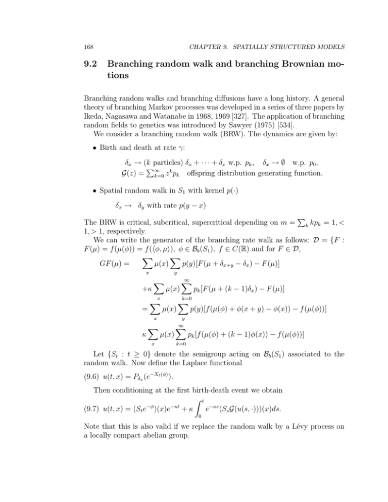
9.2 Branching random walk and branching Brownian mo- tions
advertisement

168
9.2
CHAPTER 9. SPATIALLY STRUCTURED MODELS
Branching random walk and branching Brownian motions
Branching random walks and branching diffusions have a long history. A general
theory of branching Markov processes was developed in a series of three papers by
Ikeda, Nagasawa and Watanabe in 1968, 1969 [327]. The application of branching
random fields to genetics was introduced by Sawyer (1975) [534].
We consider a branching random walk (BRW). The dynamics are given by:
• Birth and death at rate γ:
δx → (k particles) δx + · · · + δx w.p. pk , δx → ∅ w.p. p0 ,
P
k
G(z) = ∞
offspring distribution generating function.
k=0 z pk
• Spatial random walk in S1 with kernel p(·)
δx → δy with rate p(y − x)
P
The BRW is critical, subcritical, supercritical depending on m = k kpk = 1, <
1, > 1, respectively.
We can write the generator of the branching rate walk as follows: D = {F :
F (µ) = f (µ(φ)) = f (hφ, µi), φ ∈ Bb (S1 ), f ∈ C(R) and for F ∈ D,
X
X
GF (µ) =
µ(x)
p(y)[F (µ + δx+y − δx ) − F (µ)]
x
y
+κ
X
µ(x)
x
=
X
X
pk [F (µ + (k − 1)δx ) − F (µ)]
k=0
µ(x)
x
κ
∞
X
µ(x)
x
X
y
∞
X
p(y)[f (µ(φ) + φ(x + y) − φ(x)) − f (µ(φ))]
pk [f (µ(φ) + (k − 1)φ(x)) − f (µ(φ))]
k=0
Let {St : t ≥ 0} denote the semigroup acting on Bb (S1 ) associated to the
random walk. Now define the Laplace functional
(9.6) u(t, x) = Pδx (e−Xt (φ) ).
Then conditioning at the first birth-death event we obtain
Z t
−φ
−κt
(9.7) u(t, x) = (St e )(x)e + κ
e−κs (Ss G(u(s, ·)))(x)ds.
0
Note that this is also valid if we replace the random walk by a Lévy process on
a locally compact abelian group.
9.2. BRANCHING RANDOM WALK AND BRANCHING BROWNIAN MOTIONS
169
Proposition 9.7 The martingale problem for G is well posed and the Laplace
functional of the solution is the unique solution of equation (9.7).
The system of branching Brownian motions (BBM) is defined in the same way
with S = Rd with offspring produced at the location of the parent and between
branching the particles perform independent Brownian motions. (For non-local
branching see Z. Li [429].)
Remark 9.8 We sometimes combine the reproduction and spatial jump by replacing the reproduction and migration by a single mechanism in which an offspring produced by a birth immediately moves to a new location obtained by taking
a jump with kernel pε , that is, δx → δx + δy .
We also consider the N (S)-measure-valued process {Xt } in which each particle
has mass η, that is,
Xt (A) = η
N (t)
X
δxi (t) ,
A⊂S
i=1
where xi (t) denotes the location of the ith particles at time t.
Supercritical BRW and BBM
There is an important relation between supercritical branching Brownian motions
and the Fisher-KPP equation. This relation was developed by McKean [473] and
Bramson [49].
A basic question concerns the geometrical properties of the supercritical branching random walk. Biggins [38] has proved that the set I (n) of positions occupied
by nth generation individuals rescaled by a factor n1 has asymptotic shape I where
I is a convex set.
178
CHAPTER 9. SPATIALLY STRUCTURED MODELS
9.5
Measure-valued branching processes
9.5.1
Super-Brownian motion
Introduction
Super-Brownian motion (SBM) is a measure-valued branching process which generalizes the Jirina process. It was constructed by S. Watanabe (1968) [595] as
a continuous state branching process and Dawson (1975) [113] in the context of
SPDE. The lecture notes by Dawson (1993) [139] and Etheridge (2000) [217] provide introductions to measure-valued processes. The books of Dynkin [204], [205],
Le Gall [424], Perkins [514] and Li [434] provide comprehensive developments of
various aspects of measure-valued branching processes. In this section we begin
with a brief introduction and then survey some aspects of superprocesses which
are important for the study of stochastic population models. Section 9.5 gives a
brief survey of the small scale properties of SBM and Chapter 10 deals with the
large space-time scale properties.
Of special note is the discovery in recent years that super-Brownian motion
arises as the scaling limit of a number of models from particle systems and statistical physics. An introduction to this class of SBM invariance principles is
presented in Section 9.6 with emphasis on their application to the voter model
and interacting Wright-Fisher diffusions. A discussion of the invariance properties of Feller CSB in the context of a renormalization group analysis is given in
Chapter 11.
The SBM Martingale Problem
Let (D(A), A) be the generator of a Feller process on a locally compact metric space (E, d) and γ ≥ 0. The probability laws {Pµ : µ ∈ Mf (E)} on
C([0, ∞), Mf (E)) of the superprocess associated to (A, a, γ) can be characterized as the unique solution of the following martingale problem:
Z
Mt (ϕ) := hϕ, Xt i −
t
hAϕ, Xs i ds
0
is a Pµ -martingale with increasing process
Z
t
hM (ϕ)it =
γ h ϕ, Xs i ds
0
for each ϕ ∈ D(A).
9.5. MEASURE-VALUED BRANCHING PROCESSES
179
Equivalently, it solves the martingale problem
Z
δF
GF =
A
µ(dx)
δµ(x)
ZZ
γ
δ2F
+
δx (dy)µ(dx)
2
δµ(x)δµ(y)
D(G) := {F (µ) = e−µ(ϕ) , ϕ ∈ B+ (Rd )}
R
The special case E = [0, 1], Af (x) = [ f (y)ν0 (dy) − f (x)]dy is the Jirina
process. The special case E = Rd A = 21 ∆ on D(A) = Cb2 (Rd ) is called superBrownian motion.
9.5.2
Super-Brownian Motion as the Limit of Branching Brownian
Motion
Given a system of branching Brownian motions on S = Rd and ε > 0 we consider
the measure-valued process, X ε , with particle mass mε = ε and branching rate
γε = γε , that is,
ε
(9.32) X (t) = mε
N (t)
X
δxj (t)
j=1
where N (t) denotes the number of particles alive at time t and x1 (t), . . . , xN (t)
denote the locations of the particles at time t. Given an initial set of particles, let
P (0)
ε
ε
µε = mε N
j=1 δxj (0) , let Pµε denote the probability law of X on DMF (Rd ) ([0, ∞)).
Let {Ft }t≥0 be the canonical filtration on D([0, ∞), MF (Rd )).
R
Notation 9.13 µ(φ) = hφ, µi = φdµ.
Let C(MF (Rd )) ⊃ D(Gε ) := {F (µ) = f (hφ, µi)) : f ∈ Cb2 (R), φ ∈ Cb2 (Rd )}.
Then D(Gε ) is measure-determining on MF (Rd ) ([139], Lemma 3.2.5.).
Then using Itô’s Lemma, it follows that Pµεε ∈ P(D([0, ∞), MF (Rd ))) satisfies
the Gε -martingale problem where for F ∈ D(Gε ),
ε
1
Gε F (µ) = f 0 (µ(φ))µ( ∆φ) + f 00 (µ(φ))µ(∇φ · ∇φ)
2
2
Z
γ
+ 2 [f (µ(φ) + εφ(x)) + f (µ(φ) − εφ(x)) − 2f (µ(φ))]µ(dx).
2ε
Theorem 9.14 Assume that X ε (0) = µε ⇒ µ as ε → 0.
Then
ε→0
(a) Pµεε =⇒ Pµ ∈ P(CMF (Rd ) ([0, ∞)) and Pµ is the unique solution to the martingale problem: for all φ ∈ Cb2 (Rd ),
Z t
1
(9.33) Mt (φ) := Xt (φ) − µ(φ) −
Xs ( ∆φ)ds
2
0
180
CHAPTER 9. SPATIALLY STRUCTURED MODELS
is an (FtX )−martingale starting at zero with increasing process
Z t
hM (φ)it = γ
Xs (φ2 )ds.
0
(b) The Laplace functional of Xt is given by
R
R
(9.34) Pµ e(− φ(x)Xt (dx)) = e(− vt (x)µ(dx)) .
where v(t, x) is the unique solution of
(9.35)
∂v(t, x)
1
γ
= ∆v(t, x) − v 2 (t, x),
∂t
2
2
2
v0 = φ ∈ C+,b
(Rd ).
(c) The total mass process {Xt (Rd }t≥0 is a Feller CSBP.
Proof.
Step 1. Tightness of probability laws of X ε on DMF (Rd ) ([0, ∞ and a.s. continuity of limit points. In order to prove tightness it suffices to prove that for
δ > 0 there exists a compact subset K ⊂ Rd and 0 < L < ∞ such that
(9.36)
Pµεε (sup0≤t≤T Xt (K c ) > δ) < δ, Pµεε (sup0≤t≤T Xt (1) > L) < δ
and
(9.37) Pµεε ◦ (Xt (φ))−1 is tight in DR ([0, ∞)) for φ ∈ Cc2 (Rd ).
This can be checked by standard moment and martingale inequality arguments.
For example for (9.36) it suffices to show that
(9.38) sup sup E( sup he−δkxk (1 + kxk2 ), Xε (t)i) < ∞,
0<ε≤1 δ>0
0≤t≤T
and (9.37) can be verified using the Joffe-Métivier criterion (see Appendix, (17.4.2)).
The a.s. continuity of any limit point then follows from Theorem 17.14 since the
maximum jump size in X ε is ε.
Moreover, if Pµ is a limit point, it is also easy to check (cf. Lemma 16.2) that
for φ in Cb2 (Rd ), Mt (φ) is a Pµ -martingale and (F1 (µ) = µ(φ), F2 (µ) = µ(φ)2 )
Z t
hM (φ)it = lim (Gε F2 (Xs ) − 2F1 (Xs )Gε F1 (Xs ))ds
ε→0 0
Z t
= γ
Xs (φ2 )ds.
0
As pointed out above, (9.33) and Ito’s formula yields an equivalent formulation


![Branching Out: An Introduction to Family History [pptx , 2.3 MB]](http://s2.studylib.net/store/data/005232376_1-8bb1ea3bff509441ce8b545117622545-300x300.png)