Mathematics 307|September 7, 1995
Two dimensions
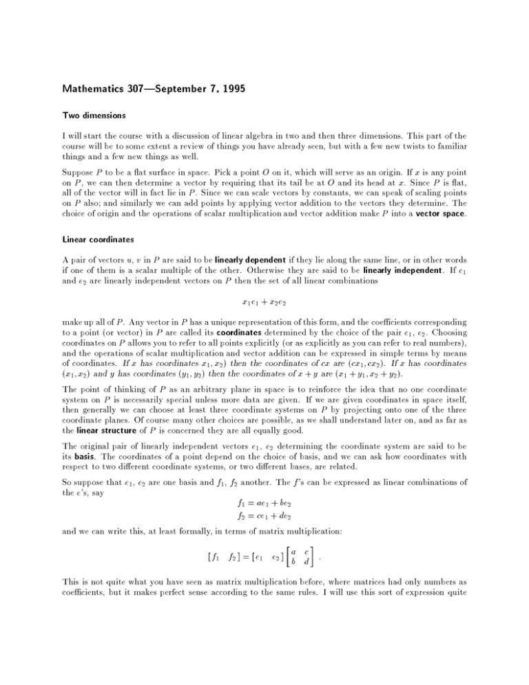
I will start the course with a discussion of linear algebra in two and then three dimensions. This part of the
course will be to some extent a review of things you have already seen, but with a few new twists to familiar
things and a few new things as well.
Suppose P to be a at surface in space. Pick a point O on it, which will serve as an origin. If x is any point
on P , we can then determine a vector by requiring that its tail be at O and its head at x. Since P is at,
all of the vector will in fact lie in P . Since we can scale vectors by constants, we can speak of scaling points
on P also; and similarly we can add points by applying vector addition to the vectors they determine. The
choice of origin and the operations of scalar multiplication and vector addition make P into a vector space.
Linear coordinates
A pair of vectors u, v in P are said to be linearly dependent if they lie along the same line, or in other words
if one of them is a scalar multiple of the other. Otherwise they are said to be linearly independent. If e1
and e2 are linearly independent vectors on P then the set of all linear combinations
x1 e1 + x2 e2
make up all of P . Any vector in P has a unique representation of this form, and the coecients corresponding
to a point (or vector) in P are called its coordinates determined by the choice of the pair e1 , e2 . Choosing
coordinates on P allows you to refer to all points explicitly (or as explicitly as you can refer to real numbers),
and the operations of scalar multiplication and vector addition can be expressed in simple terms by means
of coordinates. If x has coordinates x1; x2) then the coordinates of cx are (cx1; cx2). If x has coordinates
(x1; x2) and y has coordinates (y1 ; y2 ) then the coordinates of x + y are (x1 + y1 ; x2 + y2 ).
The point of thinking of P as an arbitrary plane in space is to reinforce the idea that no one coordinate
system on P is necessarily special unless more data are given. If we are given coordinates in space itself,
then generally we can choose at least three coordinate systems on P by projecting onto one of the three
coordinate planes. Of course many other choices are possible, as we shall understand later on, and as far as
the linear structure of P is concerned they are all equally good.
The original pair of linearly independent vectors e1 , e2 determining the coordinate system are said to be
its basis. The coordinates of a point depend on the choice of basis, and we can ask how coordinates with
respect to two dierent coordinate systems, or two dierent bases, are related.
So suppose that e1 , e2 are one basis and f1 , f2 another. The f 's can be expressed as linear combinations of
the e's, say
f1 = ae1 + be2
f2 = ce1 + de2
and we can write this, at least formally, in terms of matrix multiplication:
[ f1 f2 ] = [ e1 e2 ] ab dc :
This is not quite what you have seen as matrix multiplication before, where matrices had only numbers as
coecients, but it makes perfect sense according to the same rules. I will use this sort of expression quite
Two dimensions
2
often; I hope to show that it leads to very simple explanations of formulas that at rst sight look quite
complicated. I can write the above formula as what I call the basic equation relating two bases:
F = EA
where
F = [ f1 f2 ] ; E = [ e1 e2 ] ; A = ab dc
and the columns of A are the coordinates of the f 's in terms of the e's. We shall see later that in this
equation the 2 2 matrix A must be non-singular, which is to say that its determinant is not zero, or that
it has a matrix inverse.
This formula can be used to answer the question about dierent coordinates. Suppose x is a vector in P ,
and that E , F are two bases. Let xE and xF be the two column vectors we make up from the coordinates
of x with respect to E and F . If
xE = xx12
then we can write the equation
x = x1e1 + x2e2 = [ e1 e2 ] xx12 = ExE
and if we want to nd the column vector xF we can determine it according to the specication
x = FxF :
Well, we have
x = ExE
and also
F = EA :
We can get from this to
F = EA,1; ExE = FA,1 xE
and deduce immediately by comparison that
xF = A,1 xE :
Example. Say that
Then
since if
then
xE = 21 ; f1 = e1 + e2 ; f2 = e1 , e2 :
A = 11 ,11 ; A,1 = 11==22 ,11==22
A = ac db
d ,b
,
c a :
A,1 = det
A
Two dimensions
3
Linear transformations
A linear transformation T of P is a map from P to itself which preserves its linear structure. Geometrically,
this means that T maps parallelograms into paralleograms, and grids into (skewed) grids. Algebraically it
means that
T cx = c Tx
T (x + y) = Tx + Ty
and in terms of coordinates T must be expressed in linear terms: if x has coordinates (x1; x2) then Tx has
coordinates (ax1 + bx2; cx1 + dx2) for some constants a etc. If the coordinates of Tx are (y1 ; y2 ) we have
then a matrix equation
y1 = a b x1
y2
c d x2
or
(Tx)E = AxE
for any given basis E . The matrix is determined the formula for coordinates, but it can also be determined
by this fundamental rule: if we are given a basis E and a linear transformation T then the matrix assocaited
to T by the choice of E is the 2 2 matrix whose columns are made up of the coordinates of Te1 and Te2 .
This is because we can see that the coordinates of Te1 are
a
c
and those of Te2 are
b
d :
Examples.
The identity map
It takes any point to itself. It takes e1 to e1 and e2 to e2 . Its matrix is
1 0 :
0 1
Reection in the y-axis
It takes e1 to ,e1 , e2 to itself. The matrix is
Uniform scaling by c
It takes any x to cx. Its matrix is
,1 0 :
0 1
c 0
0 c :
Non-uniform scaling
Suppose we scale along the x-axis by a and along the y-axis by b. The matrix is
a 0 :
0 b
Two dimensions
4
Projection
A special case of scaling is where we do no scaling in the x-direction, but collapse completely vertically. This
amounts to perpendicular or orthogonal projection onto the x-axis. The matrix is
1 0 :
0 0
Rotation
Rotation in the positive direction (counter-clockwise) by has matrix
cos , sin :
sin cos Shear
Sliding parallel to the x-axis is called a horizontal shear. The matrix is of the form
1 x :
0 1