MATH 340
A Sensitivity Analysis Example from lectures
The following examples have been sometimes given in lectures and so the fractions are rather
unpleasant for testing purposes. Note that each question is imagined to be independent; the changes
are not intended to be cumulative.
We wish to consider a trucking firm who can choose to purchase three types of trucks subject to
three constraints on capital, space and number of drivers. We use variable xi to denote the number
of trucks of type i to be purchased.
Truck 1 Truck 2 Truck 3
availability
capital
24
40
46
1200 units $10K
space
1
1
1
30 trucks
drivers
3
6
6
150 people
net profit
12
20
21
Now setting xi = number of trucks of type i to be produced we have the LP:
max 12x1
24x1
x1
3x1
+20x2
+40x2
+x2
+6x2
+21x3
+46x3
+x3
+6x3
≤ 1200
≤ 30
≤ 150
x1 , x2 , x3 ≥ 0
We get the final dictionary:
x4
x1
x3
z
= 40 +2x5
= 10 −2x5
= 20 +x5
= 540 −3x5
+6x2
−x2
−x2
x
+ 22
3 6
1
+ 3 x6
− 13 x6
−3x6
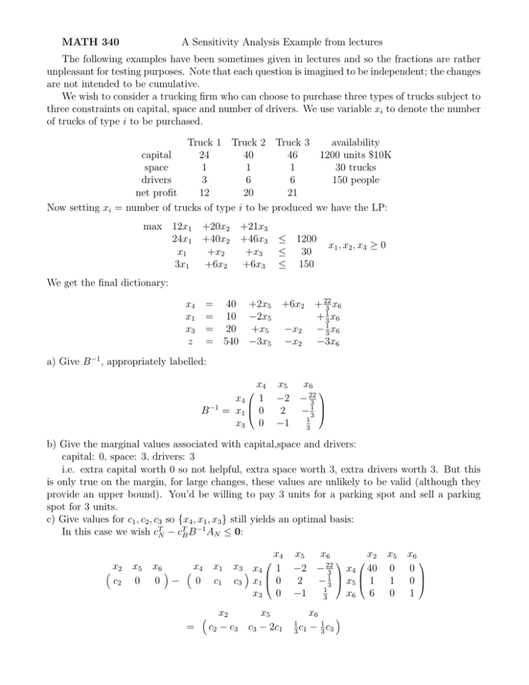
a) Give B −1 , appropriately labelled:
x4
x4 1

= x1  0
x3 0

B −1
x5
x6

−2 − 22
3
2
− 13 

1
−1
3
b) Give the marginal values associated with capital,space and drivers:
capital: 0, space: 3, drivers: 3
i.e. extra capital worth 0 so not helpful, extra space worth 3, extra drivers worth 3. But this
is only true on the margin, for large changes, these values are unlikely to be valid (although they
provide an upper bound). You’d be willing to pay 3 units for a parking spot and sell a parking
spot for 3 units.
c) Give values for c1 , c2 , c3 so {x4 , x1 , x3 } still yields an optimal basis:
In this case we wish cTN − cTB B −1 AN ≤ 0:
x2
c2
x5
0
x6 x4
0 −
0
=
x1
c1
x4

x 3 x4 1
c3 x1 
 0
x3 0
x2
c2 − c3
x5
c3 − 2c1
x5
x6
x2 x5


22
−2 − 3 x4 40 0

2
− 13 
1
 x5  1
1
−1
x6 6 0
3
1
c
3 1
x6
− 31 c3
x6

0
0

1
d) For what range on c1 is the current basis {x4 , x1 , x3 } still optimal?
1
cTN − cTB B −1 AN = [−1, 21 − 2c1 , c1 − 7) ≤ 0.
3
We deduce that 10 12 ≤ c1 ≤ 21. Note that in this range the optimal solution is x1 = 10 and x3 = 20
and so the profit would be 10c1 + 420.
e) What is the optimal solution if c1 = 10? We create the updated dictionary and try pivoting to
optimality. We believe we are close to optimal since we have made a small change.
x4
x1
x3
z
= 40 +2x5
= 10 −2x5
= 20 +x5
= ∗ +x5
+6x2
−x2
−x2
x
+ 22
3 6
+ 13 x6
− 13 x6
− 11
x
3 6
x5 enters and x1 leaves
x4
x5
x3
z
We have a new optimal solution x3
is 25 · 21 = 525, a slight reduction.
= 50
= 5
∗
= 25
x
= ∗ − 12 x1 −x2 − 11
3 6
= 25. The profit hasn’t been worked out but you can since it
f) What is the optimal solution if c1 = 22?
x4
x1
x3
z
= 40 +2x5
= 10 −2x5
= 20 +x5
= ∗ −23x5
+6x2
−x2
−x2
+ 22
x
3 6
+ 13 x6
− 13 x6
+ 13 x6
x6 enters and x3 leaves
x4 = 480
x1 = 30
∗
x6 = 60
z = ∗ −22x5 −2x2 −x3
We have a new optimal solution x1 = 30. The profit hasn’t been worked out but you can since it
is 30 · 22 = 660. We have made truck 1 valuable so we now buy lots of it.
g) For what range on c2 is the current basis optimal. We simply need c2 − cB B −1 A2 ≤ 0. Now
cB B −1 = [0, 3, 3]. So we find that for c2 ≤ 21 the the current basis (and solution) remain optimal.
h) What if we introduce a new truck (we’ll use variable x7 ) with requirements of 45 capital, 1
parking spot, 5 crew and value 22. Sounds like a winner compared with truck 3. We may imagine
adding x7 and the associated date to our original problem and compute


45


−1
c7 − cB B A7 = c7 − [ 0 3 3 ]  1  = 4.
5
Thus we would like to buy truck 7. We compute
x4
x4 1

−1
B A 7 = x1  0
x3 0

x5
x6


 1
−2 − 22
45
6
3

 13 
1 
2
−3   1  =  3 
1
2
−1
5
3
3
We insert this in our dictionary:
x4
x1
x3
z
= 40 +2x5
= 10 −2x5
= 20 +x5
= 540 −3x5
+ 22
x
3 6
+ 13 x6
− 13 x6
−3x6
+6x2
−x2
−x2
−6 13 x7
− 31 x7
− 32 x7
+4x7
Here x7 enters and x4 leaves but there is more pivoting to be done so I’ll ignore this case. Note
that since e we will have increased z above 540 then we know that track 7 will be purchased.
i) Describe a profitable truck. It is one in which 3 times the space requirement and 3 times the
labour requirement is less than the profit.
j) Determine the value of the new solution when we decrease capital by 50, increase space by 5 and
P
decrease labour by 5. Given our marginal values we expect the profit to change by i ∆bi · yi =
0 · (−5) + 3 · 5 + 3 · (−5) = 0. But this prediction works if the current basis remains feasible. Check
x4
x4 1
x1 
 0
x3 0

x5
x6
x4





22
x4 1
−2 − 3
1200 − 50
40



1 
2
− 3   30 + 5  =  10  + x1 
 0
1
−1
x3 0
150 − 5
20
3
x5
x6


 50 
−2 − 22
−50
3
3



 65
2
− 31 
  +5  =  3 
1
40
−1
−5
3
3
Thus we gently increase trucks of type 1 (to take advantage of increased parking and handle
decreased labour) while decreasing type 3.
The changes ∆b1 , ∆b2 , ∆b3 can vary quite a bit and still have B −1 ∆b ≥ 0.
k) For what values of ∆b2 is the current basis still optimal?


0

−1 
B b + ∆b2  ≥ 0
0
Thus




40
−2∆b2

 

 10  +  2∆b2  ≥ 0
20
−∆b2
from which we deduce
−5 ≤ ∆b2 ≤ 20
i.e. 25 ≤ b2 ≤ 50. The marginal value of 3 is valid in this interval.
What happens if B −1 (b + ∆b) 6≥ 0?
`) What is the optimal solution if ∆b1 = −100 and ∆b2 = 10?
We compute
x4
x4 1
−100
40




−1 
B b + 10  =  10  + x1  0
x3 0
0
20





x5
x6




−2 − 22
−100
−80
3




2
− 13 
  10  =  30  6≥ 0
1
−1
0
10
3
We would have the dictionary
x4
x1
x3
z
= −80 +2x5
= 30 −2x5
= 10
+x5
= 540 −3x5
+6x2
−x2
−x2
+ 22
x
3 6
+ 13 x6
− 13 x6
−3x6
Recall that if cTN − cTB B −1 AN ≤ 0T , and so cTB B −1 is a feasible dual solution of objective function
value cTB B −1 b. If we do not have a primal feasible solution because B −1 (b + ∆b) 6≥ 0, we still have
a dual feasible solution and so we seek to find a dual optimal solution (and so a primal optimal
solution) by minimizing the dual objective function while preserving feasibility. Following the Dual
Simplex method we have x4 leave and seek the largest λ so that
x2 x6 x5
−3 −1 −3 + λ 2 6 22
≤ 0T . We choose λ = 1/6 and so x2 enters resulting in the
3
following dictionary.
40
x2 =
− 51 x5 + 16 x4 − 11
x
3
9 6
x1 =
30
−2x5
+ 31 x6
x3 = − 10
+ 43 x5 − 16 x4 + 98 x6
3
2
x
z = 556 3 − 38 x5 − 16 x4 − 16
9 6
One more pivot required. We choose x3 to leave and then seek the largest λ so that
x4
x6 x5
8
1
4
1
8
− 3 − 6 − 16
−
+
λ
≤ 0T . There is a tie with λ = 2 and so either x5 or x6
9
3
6
9
enters but following an extended form of Anstee’s rule we choose x5 to enter. We obtain the new
dictionary (or at least the parts we need)
x2
x1
x5
z
= 25
2
= 25
5
=
2
= 550 −2x3
∗
− 12 x4
Thus we get an optimal solution (25, 25/2, 0, 0, 5/2, 0) with z = 550 (we make more money as
predicted) with new marginal values of 1/2 for capital, 0 for space, and 0 for labour.
Our tie for the entering variable results in a degeneracy in the dual.
m) What is the optimal solution if we add the constraint x2 + x3 ≥ 15? First note that adding a
constraint can only decrease the value of the objective function (it may even make the LP ifeasible).
The answer here is easy. Our current solution x1 = 10 and x3 = 20 with z = 540 remains optimal.
n) What is the optimal solution if we add the constraint x2 + x3 ≥ 22?
We start by noting that our current optimal solution is not feasible. So we have to do something.
We add a new slack variable x7 = x2 + x3 − 22. We can’t introduce this directly into our dictionary
because it contains a basic variable but we can express x3 in terms of non-basic variables and obtain
1
1
x7 = x2 + x3 − 22 = x2 + (20 + x5 − x2 − x6 ) − 22 = −2 + x5 − x6
6
6
We have the dictionary
x4
x1
x3
x7
z
= 40 +2x5
= 10 −2x5
= 20 +x5
= −2 +x5
= 540 −3x5
+6x2
−x2
−x2
+ 22
x
3 6
1
+ 3 x6
− 13 x6
− 16 x6
−3x6
We follow the dual simplex algorithm, attempting to decrease z value while maintaining dual
feasibility by having x7 leave the basis.
x
x2 x 6 5
−3 −1 −3 + λ 1 0 − 16 ≤ 0T . We can take λ = 3 and choose x5 as the entering
variable. Our new dictionary is:
x4
x1
x3
x5
z
= 44
= 6
= 22
= 2
= 534 −3x7
∗
−x2
−4x6
We have a new optimal solution x1 = 6 and x3 = 22 (thus we satisfy the constraint x2 + x3 ≥ 22)
with z = 534 (a reduction in profitability from the added constraint). The marginal values are 0
fro capital, 0 for space, 4 for labour and 3 for the new constraint. We assume the new constraint
is written as −x2 − x3 ≤ −22 and so increasing −22 to −21 results in less of a restriction and so
an expectation of increased profit of 3 units. When LINDO is given the constraint explicitly as
x2 + x3 ≥ 22 it will return a dual price of −3 so that if you increase 22 to 23 then you expect profit
to drop by 3.
After n questions perhaps you don’t need anymore but we discussed in class two questions:
o) How do we delete a variable? Two suggestions were offered. If for example we wished to remove
x3 we could set c3 = −1, making x3 unprofitable and our sensitivity techniques would drive it to
0. We could add a constraint x3 = 0 (or x3 ≤ 0) and proceed as above. If we wished to remove x2 ,
since it is non-basic we could just delete it from further consideration.
p) How do we delete a constraint? If for example we wished to remove x1 + x2 + x3 ≤ 30 we
could simply change the right hand side to some large number (say 1000) essentially eliminating
the constraint. Or we could add a variable to the constraint x1 + x2 + x3 − x7 ≤ 30 where c7 = 0.
If the constraint is currently non-binding, such as capital, then essentially the constraint has been
eliminated.
q) How do we change an entry in A? This is more difficult but still possible. For the column of a
nonbasic variable this is reasonable (try it!). In a test environment, only one pivot suffices to get
you to optimality but this is unrealistic and for some changes it may be advisable to start from
scratch.