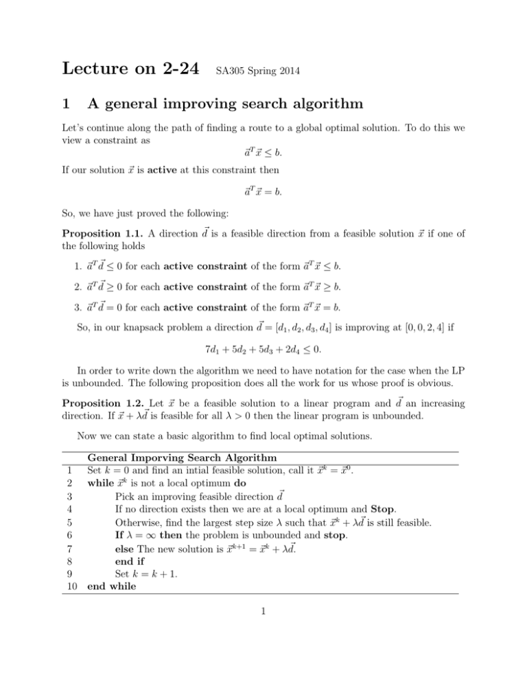
Lecture on 2-24 1 A general improving search algorithm
advertisement

Lecture on 2-24
1
SA305 Spring 2014
A general improving search algorithm
Let’s continue along the path of finding a route to a global optimal solution. To do this we
view a constraint as
~aT ~x ≤ b.
If our solution ~x is active at this constraint then
~aT ~x = b.
So, we have just proved the following:
Proposition 1.1. A direction d~ is a feasible direction from a feasible solution ~x if one of
the following holds
1. ~aT d~ ≤ 0 for each active constraint of the form ~aT ~x ≤ b.
2. ~aT d~ ≥ 0 for each active constraint of the form ~aT ~x ≥ b.
3. ~aT d~ = 0 for each active constraint of the form ~aT ~x = b.
So, in our knapsack problem a direction d~ = [d1 , d2 , d3 , d4 ] is improving at [0, 0, 2, 4] if
7d1 + 5d2 + 5d3 + 2d4 ≤ 0.
In order to write down the algorithm we need to have notation for the case when the LP
is unbounded. The following proposition does all the work for us whose proof is obvious.
Proposition 1.2. Let ~x be a feasible solution to a linear program and d~ an increasing
direction. If ~x + λd~ is feasible for all λ > 0 then the linear program is unbounded.
Now we can state a basic algorithm to find local optimal solutions.
General Imporving Search Algorithm
1 Set k = 0 and find an intial feasible solution, call it ~xk = ~x0 .
2 while ~xk is not a local optimum do
3
Pick an improving feasible direction d~
4
If no direction exists then we are at a local optimum and Stop.
5
Otherwise, find the largest step size λ such that ~xk + λd~ is still feasible.
6
If λ = ∞ then the problem is unbounded and stop.
~
7
else The new solution is ~xk+1 = ~xk + λd.
8
end if
9
Set k = k + 1.
10 end while
1
However there is a lot missing from this algorithm:
1. We do not know how to find an initial feasible solution.
2. We do not know how to find an improving direction.
3. We do not know how to find the step sizes.
On the other hand we do have the following Proposition that says this algorithm works.
Proposition 1.3. Under certain assumptions this algorithm will find a local optimal solution.
2
Convexity
Now the above discussion is sort of lame! Because we do not care about local optimal
solutions, we care about global optimal solutions! However, there is the amazing restriction
to convex things that makes everything easy. To do this let’s write a definition.
Definition 2.1. A subset S ⊆ Rn is convex if for all ~x, ~y ∈ S and for all λ ∈ [0, 1] the
vectors
λ~x + (1 − λ)~y ∈ S.
This means that for all points in the space S the line between the points is contained
entirely in S. The next theorem is the main point of this section, the proof is easy.
Theorem 2.2. If a linear program is asking to maximize/minimize a linear function, the
feasible region is convex, and the General Improving Search Algorithm has found a local
optimal solution ~y then ~y is actually a global optimal solution.
This theorem is true in more generality which is important for us. To state it we need a
little more notation.
Definition 2.3. Let {~v1 , . . . , ~vk } be a set of solutions in Rn . Then ~x is a convex combination
of these solutions if there exists constants {α1 , . . . , αk } ⊆ [0, ∞) that satisfy
k
X
αi = 1
i=1
such that
~x =
k
X
αi~vi .
i=1
Now we construct the general form of our feasible regions in linear programs.
2
Definition 2.4. Let {~v1 , . . . , ~vk } be a set of solutions in Rn . The convex hull of {~v1 , . . . , ~vk }
denoted by
conv({~v1 , . . . , ~vk })
is the set of all convex combinations of {~v1 , . . . , ~vk }.
Then the following proposition characterizes the convex hull of any finite set in the terms
that we need.
Proposition 2.5. The convex hull of any finite set can be written as a set of linear inequalities.
Now we’d like to optimize over a functions where our main theorem is true over convex
feasible regions. These function are exactly the following type.
Definition 2.6. Let S ⊆ Rn be a convex set. A function f (~x) is convex/concave on S if for
all ~x, ~y ∈ S and for all λ ∈ [0, 1]
f (λ~x + (1 − λ)~y ) ≤ λf (~x) + (1 − λ)f (~y )
for convex and
f (λ~x + (1 − λ)~y ) ≥ λf (~x) + (1 − λ)f (~y )
for concave.
The following proposition tells us that our linear functions that we are usually optimizing
is just a special case of these convex and concave functions.
Proposition 2.7. If f is a linear function on a convex set S then f is both concave and
convex on S.
Now we can rephrase our main theorem in terms of convex and concave functions.
Theorem 2.8. Let S ⊆ Rn be a convex set.
1. Let f (~x) be a convex function on S. If an improving search algorithm stops at a local
maximum ~y then ~y is actually a global optimum.
2. Let f (~x) be a concave function on S. If an improving search algorithm stops at a local
minimum ~y then ~y is actually a global optimum.
To finish off our discussion of convexity we will put it more into the context of a linear
program. To do this we need the following definitions.
Definition 2.9.
1. A half space of Rn is a space of the form
{~x ∈ Rn |~aT ~x ≤ k}
which is one of the halves that the hyperplane given by the equation ~aT ~x = k splits
Rn into.
3
2. A polyhedron or a polyhedral set is a subset of Rn that is the intersection of a finite
number of half spaces.
3. A polytope is a bounded polyhedron.
Proposition 2.10. If S is a polyhedral set then S is convex.
In all the linear programs that we have seen the feasible regions are all polyhedrons and
hence convex. So, that means that all are problems can be solved with our general improving
algorithm to find a global optimal solution.
4


