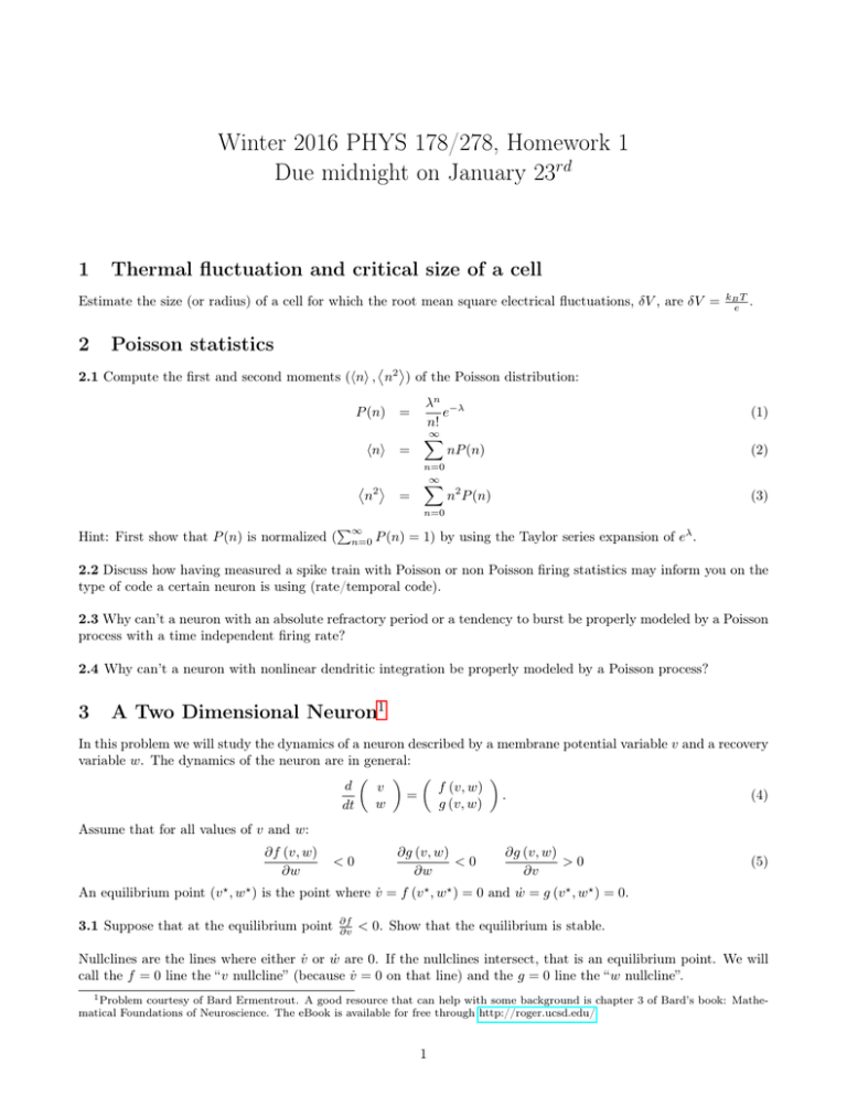
Winter 2016 PHYS 178/278, Homework 1
Due midnight on January 23rd
1
Thermal fluctuation and critical size of a cell
Estimate the size (or radius) of a cell for which the root mean square electrical fluctuations, δV , are δV =
2
kB T
e
.
Poisson statistics
2.1 Compute the first and second moments (hni , n2 ) of the Poisson distribution:
P (n)
=
hni =
2
n
=
λn −λ
e
n!
∞
X
nP (n)
n=0
∞
X
(1)
(2)
n2 P (n)
(3)
n=0
P∞
Hint: First show that P (n) is normalized ( n=0 P (n) = 1) by using the Taylor series expansion of eλ .
2.2 Discuss how having measured a spike train with Poisson or non Poisson firing statistics may inform you on the
type of code a certain neuron is using (rate/temporal code).
2.3 Why can’t a neuron with an absolute refractory period or a tendency to burst be properly modeled by a Poisson
process with a time independent firing rate?
2.4 Why can’t a neuron with nonlinear dendritic integration be properly modeled by a Poisson process?
3
A Two Dimensional Neuron1
In this problem we will study the dynamics of a neuron described by a membrane potential variable v and a recovery
variable w. The dynamics of the neuron are in general:
d
v
f (v, w)
=
.
(4)
w
g (v, w)
dt
Assume that for all values of v and w:
∂f (v, w)
∂w
<0
∂g (v, w)
<0
∂w
∂g (v, w)
>0
∂v
(5)
An equilibrium point (v ? , w? ) is the point where v̇ = f (v ? , w? ) = 0 and ẇ = g (v ? , w? ) = 0.
3.1 Suppose that at the equilibrium point
∂f
∂v
< 0. Show that the equilibrium is stable.
Nullclines are the lines where either v̇ or ẇ are 0. If the nullclines intersect, that is an equilibrium point. We will
call the f = 0 line the “v nullcline” (because v̇ = 0 on that line) and the g = 0 line the “w nullcline”.
1 Problem courtesy of Bard Ermentrout. A good resource that can help with some background is chapter 3 of Bard’s book: Mathematical Foundations of Neuroscience. The eBook is available for free through http://roger.ucsd.edu/
1
Figure 1: Sketch of v, w nullclines.
A specific model
We will work with the Fitzhugh-Nagumo model:
f (v, w)
g (v, w)
1
= v − v3 − w + I
3
= φ (av − w)
(6)
(7)
3.2 Plot the nullclines of the model (solve for w(v) such that f or g are 0, see sketch below) for the parameters
I = 3, a = 2. Note that the v nullcline has three “branches” and the w nullcline is monotonic.
3.3 Find parameters such that the equilibrium is in the middle branch of the v nullcline. Compute ∂f
∂v at the
equlibrium and show that it is positive. Given your answer to 2.1. what does that say about the equilibrium point?
3.4 Now find two sets of parameters and plot the nullclines for each of them:
• one such that the equilibrium is in the middle branch of the v nullcline and the slope of the v nullcline is
smaller than the slope of the w nullcline at the equilibrium point.
• another such that the equilibrium is in the middle branch of the v nullcline and the slope of the v nullcline
is greater than the slope of the w nullcline at the equilibrium point.
Use linear stability analysis to show that in the first case the equilibrium is a node and that in the second case it
is a saddle. Can you use the nullcline plots to explain this graphically?
3.5 (Bonus) Run the dynamics. Plot example spike trains and discuss the different regimes you identified above.
A general model (Bonus)
Assume the v nullcline has a cubic shape and the w nullcline is monotonically increasing (see sketch).
3.6 Prove that if there is an equilibrium point in the middle branch of the v nullcline then ∂f
∂v > 0.
3.7 Suppose there is a middle branch equilibrium. Prove that the equlibrium is a saddle if the slope of the w
nullcline is less than the slope of the v nullcline; and that the equilibrium is a node if the slope of the w nullcline
is greater than the slope of the v nullcline.
2