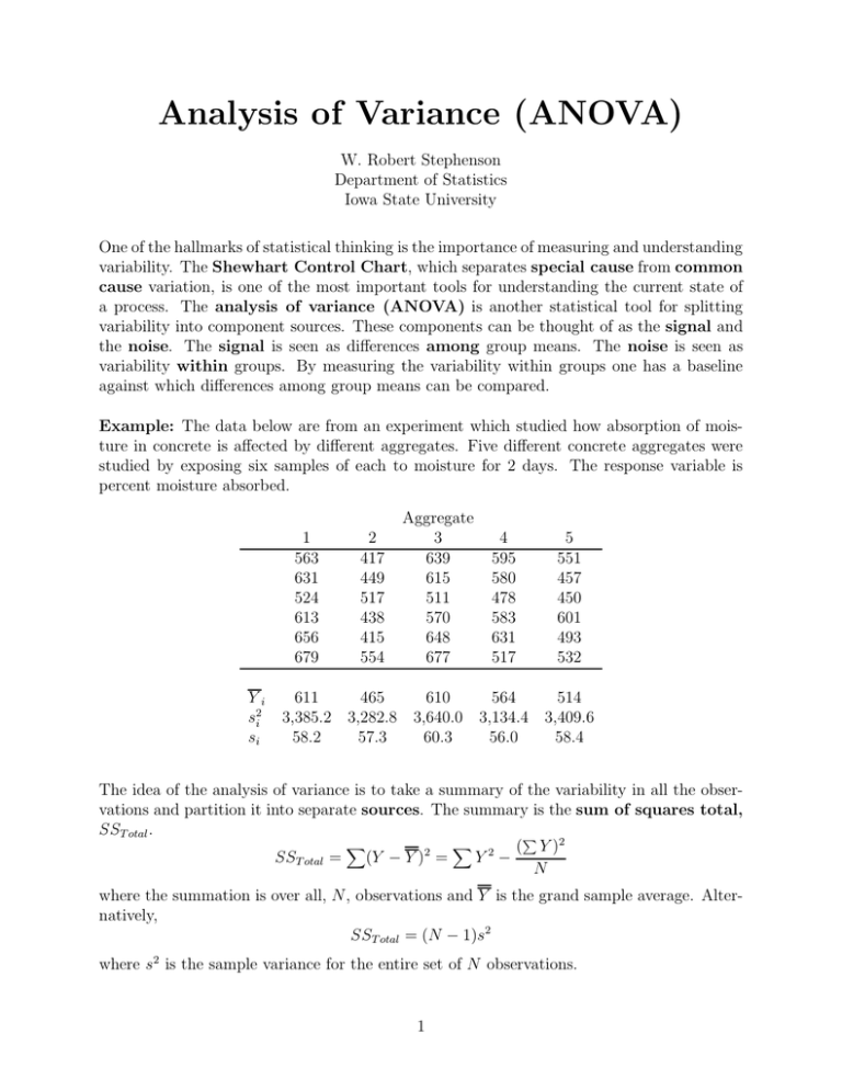
Analysis of Variance (ANOVA)
W. Robert Stephenson
Department of Statistics
Iowa State University
One of the hallmarks of statistical thinking is the importance of measuring and understanding
variability. The Shewhart Control Chart, which separates special cause from common
cause variation, is one of the most important tools for understanding the current state of
a process. The analysis of variance (ANOVA) is another statistical tool for splitting
variability into component sources. These components can be thought of as the signal and
the noise. The signal is seen as differences among group means. The noise is seen as
variability within groups. By measuring the variability within groups one has a baseline
against which differences among group means can be compared.
Example: The data below are from an experiment which studied how absorption of moisture in concrete is affected by different aggregates. Five different concrete aggregates were
studied by exposing six samples of each to moisture for 2 days. The response variable is
percent moisture absorbed.
1
563
631
524
613
656
679
Yi
s2i
si
2
417
449
517
438
415
554
Aggregate
3
639
615
511
570
648
677
4
595
580
478
583
631
517
5
551
457
450
601
493
532
611
465
610
564
514
3,385.2 3,282.8 3,640.0 3,134.4 3,409.6
58.2
57.3
60.3
56.0
58.4
The idea of the analysis of variance is to take a summary of the variability in all the observations and partition it into separate sources. The summary is the sum of squares total,
SST otal .
( Y )2
2
2
Y −
SST otal = (Y − Y ) =
N
where the summation is over all, N, observations and Y is the grand sample average. Alternatively,
SST otal = (N − 1)s2
where s2 is the sample variance for the entire set of N observations.
1
Example:
N=30
Y = 16,584
Y = 552.8
SST otal = [9, 347, 888 −
Y 2 = 9,347,888
(16, 584)2
] = 180, 252.8
30
This sum of squares total is partitioned into two separate, and additive, pieces. These
are a sum of squares among, SSAmong and a sum of squares within, SSW ithin . The
SSW ithin accumulates variability from within each group.
SSW ithin =
(ni − 1)s2i
where s2i is the sample variance of the ith group and ni is the number of observations in the
ith group.
Example:
SSW ithin = 5(3, 384.2) + 5(3, 282.8) + 5(3, 640.0) + 5(3, 134.4) + 5(3409.6) = 84, 260
The sum of squares among, SSAmong measures variability due to differences among the
group means.
SSAmong =
ni (Y i − Y )2
where Y i is the sample mean for the ith group.
Example:
SSAmong = 6(611 − 552.8)2 + 6(465 − 552.8)2 + 6(610 − 552.8)2
+ 6(564 − 552.8)2 + 6(514 − 552.8)2
= 6(58.2)2 + 6(−87.8)2 + 6(57.2)2 + 6(11.2)2 + 6(−38.8)2
SSAmong = 95,992.8
Note that SSAmong + SSW ithin = SST otal .
Associated with each sum of squares is a degrees of freedom. In general, one starts
with N degrees of freedom and loses one degree of freedom for every sample mean calculated. For the SST otal there is one grand sample average, therefore there are N − 1 degrees
of freedom. There are ni − 1 degrees of freedom within each group. Therefore, there are
(ni − 1) = N − k degrees of freedom for SSW ithin . That leaves k − 1 degrees of freedom
for SSAmong .
2
A sum of squares divided by its associated degrees of freedom produces a mean square.
The sums of squares, degrees of freedom, and mean squares are all summarized in an analysis
of variance (ANOVA) table.
Example:
Source of Variation Sum of Squares
Degrees of Freedom
Mean Square
Among
95,992.8
4
23,998.2
Within
84,260.0
25
3,370.4
Total
180,252.8
29
Each mean square captures different elements of variability. The mean square within is often
referred to as the mean square error. Within sample variability is attributed to random
(sampling) error. This is the baseline against which differences among group means are compared. The mean square among contains some of this error variability but also variability
M SAmong
due to differences among group means. The ratio F = M SW
serves as a measure of the
ithin
statistical importance or significance of the differences among the group means. Values
of F close to one indicate that the differences among group means can be attributed to
natural or random error variability. Values of F much larger than one indicate that some of
the groups differ significantly in terms of their mean or average values. The cutoff between
“close to one” and “much larger than one” can be found in a table of the F distribution. This
tabulation assumes that the original observations are normally distributed with a common
error variance.
Example:
F =
23, 998.2
= 7.12
3, 370.4
A critical value of F with 4 degrees of freedom for the numerator and 25 degrees of freedom
for the denominator is 2.76. Since 7.12 is greater than this critical value, one concludes that
some of the concrete aggregates differ significantly in terms of the absorption of moisture.
However, at this point we do not know where those differences may lie. Significance for the
analysis of variance should be followed up with some form of multiple comparison like the
Least Significant Difference.
3