Electronic Journal of Differential Equations, Vol. 2008(2008), No. 140, pp. 1–8.
ISSN: 1072-6691. URL: http://ejde.math.txstate.edu or http://ejde.math.unt.edu
ftp ejde.math.txstate.edu (login: ftp)
ASYMPTOTIC BEHAVIOR OF A DELAY PREDATOR-PREY
SYSTEM WITH STAGE STRUCTURE AND VARIABLE
COEFFICIENTS
ERIC AVILA-VALES, ANGEL G. ESTRELLA, JAVIER A. HERNANDEZ-PINZON
Abstract. In this paper, we establish a global attractor for a Lotka-Volterra
type reaction-diffusion predator-prey model with stage structure for the predator, delay due to maturity and variable coefficients. This attractor is found by
the method of upper and lower solutions and is given in terms of bounds for
the coefficients.
1. Introduction
Almost all animals have the stage structure of immature and then mature, and
in each stage they show different characteristics. For instance, immature predators
are not able to hunt, while mature animals have more powerful survival capacities;
likewise, rates of birth or death vary on each stage. Therefore, considering stagestructured models could lead to more accurate results.
In 2006, Xu, Chaplain and Davidson [7], considered the following Lotka-Volterra
type reaction-diffusion predator-prey model with stage structure for the predator
and delay due to maturity
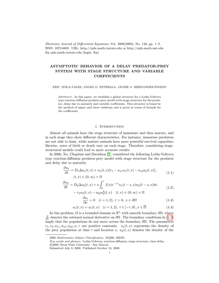
∂u1
= D1 ∆u1 (t, x) + u1 (t, x)[r1 − a11 u1 (t, x) − a12 u2 (t, x)],
∂t
(1.1)
(t, x) ∈ (0, ∞) × Ω
Z τ
∂u2
= D2 ∆u2 (t, x) + α
f (s)e−γs u1 (t − s, x)u2 (t − s, x)ds
∂t
(1.2)
0
− r2 u2 (t, x) − a22 u22 (t, x) (t, x) ∈ (0, ∞) × Ω
∂ui
= 0 (i = 1, 2), t > 0, x ∈ ∂Ω
∂ν
ui (t, x) = φi (t, x) (i = 1, 2), t ∈ [−τ, 0] , x ∈ Ω
(1.3)
(1.4)
In this problem, Ω is a bounded domain in Rn with smooth boundary ∂Ω, where
denotes the outward normal derivative on ∂Ω. The boundary conditions in (1.3)
imply that the populations do not move across the boundary ∂Ω. The parameters
r1 , r2 , a11 , a12 , a22 , α, γ are positive constants. u1 (t, x) represents the density of
the prey population at time t and location x, u2 (t, x) denotes the density of the
∂
∂ν
2000 Mathematics Subject Classification. 35Q80, 92D25.
Key words and phrases. Lotka-Volterra; reaction-diffusion; stage structure; time delay.
c
2008
Texas State University - San Marcos.
Submitted July 8, 2008. Published October 16, 2008.
1
2
E. AVILA-V., A. G. ESTRELLA, J. A. HERNANDEZ-P.
EJDE-2008/140
mature predator population at time t and location x, respectively. The data φi (t, x)
i
(i = 1, 2) are nonnegative and Hölder continuous and satisfy ∂φ
∂ν = 0 in (−τ, 0)×∂Ω.
The model is derived under the following assumptions.
• The prey population: The growth of the species is of Lotka - Volterra nature. The parameters r1 , a11 and D1 are the intrinsic growth rate, intra-specific
competition rate and diffusion rate, respectively.
• The predator population: a12 , aα12 , r2 and a22 are the capturing rate, conversion
rate,death rate and intra-specific competition rate of the mature predator, respectively; γ > 0 is the death rate of the immature predator population, D2 is the
diffusion rate of the mature population. The term αu1 (t − s, x)u2 (t − s, x) is the
number born at time t−s and location x per unit time, and is taken as proportional
to the number of the prey and mature predator the around. f (s) denotes the probthat the maturation time is between s and s + ds with ds infinitesimal,and
Rability
∞
f
(s)ds
= 1. e−γs is the probability of an individual born at time t − s still alive
0
at time t. Individuals becoming mature at time t could have been born at any time
prior to this, and the integral totals up the contributions from all previous times.
They also use the following assumptions:
(H1) Rf (t) is piecewise continuous in [0, τ ] and has the property: f (t) ≥ 0,
τ
f (t)dt = 1; i.e., f (t) is a probability diet on [0, τ ]
0
System (1.1)–(1.4) possesses a trivial uniform equilibrium E0 (0, 0) and a semi-trivial
1
, 0 . If the following holds:
uniform equilibrium E1 ar11
(H2) r1 αI > r2 a11 .
Then (1.1)–(1.4) also has a unique positive uniform equilibrium E ? (u?1 , u?2 ) where:
u?1 =
where I =
Rτ
0
r1 a22 + r2 a12
,
a11 a22 + αa12 I
u?2 =
r1 αI − r2 a11
a11 a22 + αa12 I
(1.5)
f (s)e−γs ds. The main result in [7] is as follows:
Theorem 1.1. Let the initial functions φi (i = 1, 2) be Hölder continuous in
[−τ, 0] × Ω, with φi (t, x) ≥ 0, φi (0, x) 6= 0. Let (u1 (t, x), u2 (t, x)) satisfy (1.1)–
(1.4). In addition to (H1)–(H2), assume that
Rτ
(H3) a11 a22 > a12 α 0 f (s)e−γs ds
Then limt→∞ ui (t, x) = u?i (i = 1, 2) uniformly for x ∈ Ω
Xu, Chaplain and Davidson considered both, the coefficients of inter-species interaction and their birth and death rates to be constant. However, it must not be
forgotten that the variability implicit in the environment means that these coefficients may depend on variables such as time, temperature, light flux, etc. Therefore,
whenever possible, it is convenient to introduce these factors as functions of these
variables even though this may complicate the resolution of the system of differential equations [4].
EJDE-2008/140
ASYMPTOTIC BEHAVIOR
3
In this work, we extend Theorem 3.3 to the case where the coefficients are functions of space and time as follows
∂u1
= D1 ∆u1 (t, x) + u1 (t, x) r1 (t, x) − a11 (t, x)u1 (t, x) − a12 (t, x)u2 (t, x)
∂t
(1.6)
Z τ
∂u2
= D2 ∆u2 (t, x) + α(t, x)
f (s)e−γs u1 (t − s, x)u2 (t − s, x)ds
∂t
(1.7)
0
− r2 (t, x)u2 (t, x) − a22 (t, x)u22 (t, x); (t, x) ∈ (0, ∞) × Ω
∂ui
= 0 (i = 1, 2), t > 0, x ∈ ∂Ω
∂ν
ui (t, x) = φi (t, x) (i = 1, 2), t ∈ [−τ, 0], x ∈ Ω
(1.8)
(1.9)
In our case the asymptotic behavior of time-dependent solution will be determined since we will be able to a obtain a prior upper an lower bounds for the system
(1.6)–(1.9).
Similar problems with constant coefficients are considered in [2, 8], where systems
of equations with diffusion are studied. One equation with diffusion and variable
coefficients is analyzed in [9]. The competition case with diffusion and variable
coefficients is studied in [6]. Some cases of variable coefficients with no diffusion
are studied in [1, 5, 10].
The rest of the paper is organized as follows. In section 2 we state the definition of
upper and lower solutions, we also discuss the existence and uniqueness of positive
solution of our system. In section 3 we find a global attractor for (1.6)–(1.9).
Finally, we present a brief discussion in the last section.
2. Preliminaries
Definition 2.1. A pair of functions
ũ(t, x) = (ũ1 (t, x), ũ2 (t, x)),
û(t, x) = (û1 (t, x), û2 (t, x))
defined for t ≥ 0, x ∈ Ω are called coupled upper and lower solutions of systems
(1.6)–(1.9) if ũi ≥ ûi in [−τ × Ω) and if for all ψi such that ûi ≤ ψi ≤ ũi the
following differential inequalities hold:
∂ ũ1
≥ D1 ∆ũ1 + ũ1 (t, x)[r1 (t, x) − a11 (t, x)ũ1 (t, x) − a12 (t, x)û2 (t, x)]
∂t
Z τ
∂ ũ2
≥ D2 ∆ũ2 (t, x) + α(t, x)
f (s)e−γs ψ1 ψ2 ds − r2 (t, x)ũ2 − a22 (t, x)ũ22
∂t
0
∂ û1
≤ D1 ∆û1 + û1 (t, x)[r1 (t, x) − a11 (t, x)û1 − a12 (t, x)ũ2 ]
∂t
Z τ
∂ û2
≤ D2 ∆û2 (t, x) + α(t, x)
f (s)e−γs ψ1 ψ2 ds
∂t
0
− r2 (t, x)ũ2 (t, x) − a22 (t, x)(ũ2 (t, x))2
for (t, x) ∈ (0, ∞) × Ω, and
∂ ûi
∂ ũi
≤0≤
(i = 1, 2), (t, x) ∈ (0, ∞) × ∂Ω
∂ν
∂ν
ûi (t, x) ≤ φi (t, x) ≤ ũi (t, x) (i = 1, 2), (t, x) ∈ [−τ, 0] × Ω
4
E. AVILA-V., A. G. ESTRELLA, J. A. HERNANDEZ-P.
EJDE-2008/140
It is easy to see that (0, 0) and (k1 , k2 ), with
r1
k1 = max{
, sup kφ(θ, ·)k},
A11 −τ ≤θ≤0
r
Rτ 2
k2 = max{
, sup kφ(θ, ·)k},
α2 k1 0 f (s)e−γτ dτ −τ ≤θ≤0
are pairs of coupled lower-upper solutions of problem (1.6)–(1.9).
The existence of solutions of problem (1.6)–(1.9) is guaranteed by a result established by Redlinger in [3] if the reaction part of the equations satisfy the Lipschitz
condition, which turns to be true in this case.
Proposition 2.2. Let the initial function φ be Hölder continuous in [−τ, 0] × Ω.
Assume that A1 ≥ 0, B > 0, A2 > 0, and f (s) is defined as in (H1). Let u(x, t) be
a nonnegative nontrivial solution of the scalar problem
Z τ
∂u
= D∆u + B
f (s)e−γs u(t − s, x)ds − A1 u(t, x) − A2 u2 (t, x), (t, x) × Ω,
∂t
0
∂u
= 0, (t, x) × ∂Ω,
∂ν
u(t, x) = φ(t, x) ≥ 0, φ(0, x) 6= 0, (t, x) ∈ [−τ, 0] × Ω.
Then we have
Rτ
(i) if B 0 f (s)e−γs ds > A1 , then
Rτ
B 0 f (s)e−γs ds − A1
lim u(t, x) =
t→∞
A2
Rτ
−γs
(ii) if B 0 f (s)e
ds < A1 , then
lim u(t, x) = 0
t→∞
uniformly for x ∈ Ω
uniformly for x ∈ Ω
A proof of the above proposition can be found in [7].
3. Global Attractor
We assume that system (1.6)–(1.9) has bounded variable coefficients with the
following properties:
0 < a11 ≤ a11 (t, x) ≤ A11 ,
0 < r1 ≤ r1 (t, x) ≤ R1 ,
0 ≤ α1 ≤ α(t, x) ≤ α2 ,
0 < a12 ≤ a12 (t, x) ≤ A12 ,
0 < r2 ≤ r2 (t, x) ≤ R2 ,
0 < a22 ≤ a22 (t, x) ≤ A22 .
We have the following results.
Proposition 3.1. Let u1 , u2 be solutions of (1.6)–(1.9),
M i = lim inf [min ui (t, x)],
t→∞
Rτ
x∈Ω
M i = lim sup[max ui (t, x)]
t→∞
x∈Ω
−γs
ds. Assume (H1), and that the initial conditions φi ≥ 0 for
and I = 0 f (s)e
i = 1, 2.
(a) If M 1 > αR12I , then
α1 M 1 I − R2
α2 M 1 I − r2
≤ M2 ≤ M2 ≤
A22
a22
(3.1)
EJDE-2008/140
ASYMPTOTIC BEHAVIOR
5
(b) If a11 r2 ≥ α2 R1 I, then M 2 = 0 = M2 .
Proof. Let ū and û be solutions of
L2 ū = α2 M1 I(ū) − r2 ū − a22 ū2 ,
L2 û = α1 M 1 I(û) − R2 û − A22 û2 ,
(3.2)
with boundary conditions and initial values as for u2 , where Li u = ut − Di ∆u for
i = 1, 2, and
Z τ
I(u) =
f (s)e−γs u(t − s, x)ds,
0
then ū and û are upper and lower solutions of u2 ; therefore
û ≤ u2 ≤ ū.
If M 1 >
R2
α1 I
then M 1 >
r2
α2 I ,
(3.3)
thus applying (a) of Proposition 2.2 we obtain
α1 M 1 I − R2
α2 M 1 I − r2
, lim ū =
,
t→∞
t→∞
A22
a22
from this and (3.3) we obtain (3.1). The proof of de second part is similar using
(b) of Proposition 2.2.
lim û =
With a similar idea and taking the appropriate upper and lower solutions of (1.6)
we note that
R1 − M 2 a12
r1 − M 2 A12
≤ M1 ≤ M1 ≤
.
(3.4)
A11
a11
With the hypothesis and notation of the previous proposition and its proof, we
have the following result.
Proposition 3.2. If a11 r2 ≤ α2 R1 I, then
M2 ≤
α2 aR111 I − r2
a22
(3.5)
Proof. ¿From equation (3.4) we have that M 1 < R1 /a11 , therefore for each > 0
there exists T > 0 such that u1 (t − s, x) < (R1 /a11 ) + for all t > T , s ∈ [0, τ ] and
x ∈ Ω. Let ω2 be a solution of
R1
+ ε I(ω2 )(t, x) − r2 ω2 (t, x) − a22 (ω2 (t, x))2 ; t > T, x ∈ Ω (3.6)
L2 ω2 = α2
a11
∂ω2
= 0 t > T, x ∈ ∂Ω
(3.7)
∂t
ω2 (t, x) = k2 (t, x) ∈ [T − τ, T ] × Ω.
(3.8)
R∞
where I(w)(t, x) = 0 f (s)e−γs w(t − s, x)ds. Since
R1
R1
α2
+ ε I ≥ α2
I ≥ r2
a11
a11
then we can use Proposition 2.2 to obtain
α2 aR111 + ε I − r2
.
lim ω2 (t, x) =
t→∞
a22
Since ω2 is an upper solution of u2 , ω2 (t, x) ≤ u2 (t, x) for t > T and x ∈ Ω; therefore
α2 aR111 + ε I − r2
M 2 ≤ lim ω2 (t, x) =
t→∞
a22
6
E. AVILA-V., A. G. ESTRELLA, J. A. HERNANDEZ-P.
EJDE-2008/140
and we obtain (3.5) from the fact that is arbitrary.
Now, we are able to state our two main results.
Theorem 3.3. Let the initial functions φi be Hölder continuous in [−τ, 0] × Ω,
with φi (t, x) ≥ 0, φi (0, x) 6= 0 for i = 1, 2. Let u1 (t, x), u2 (t, x) satisfy (1.6)–(1.9).
In addition to (H1) assume further that
a11 r2 ≤ α2 R1 I,
(3.9)
α2 A12 R1 I ≤ a11 (a22 r1 + a12 r2 ) .
(3.10)
α1 IM 1 − A22 M 2 ≤ R2 ,
(3.11)
r2 ≤ α2 IM 1 − a22 M 2 ,
(3.12)
r1 ≤ A11 M 1 + A12 M 2 ,
(3.13)
a11 M 1 + a12 M 2 ≤ R1 .
(3.14)
Then
Proof. From (3.10) we obtain
α2 aR111 I − r2
r1 −
A11 R2
α1 I
≤
.
a22
A12
Now, we can use Proposition 3.2, because of (3.9), the above inequality leads to
M2 ≤
r1 −
A11 R2
α1 I
A12
which implies
r1 − M 2 A12
R2
≤
α1 I
A11
and with (3.4), we obtain
R2
≤ M 1,
α1 I
thus, we can use Proposition 3.1 to obtain (3.11)–(3.12), and (3.13)–(3.14) follow
from (3.4).
Theorem 3.4. Let δ = a11 a22 A11 A22 −a12 A12 α1 α2 I 2 , and assume hypothesis (H1)
and (3.9)–(3.10). If δ > 0, then
s1 ≤ M 1 ≤ M 1 ≤ S1 ,
s2 ≤ M 2 ≤ M 2 ≤ S2 ,
where
a11 A22 (A12 r2 + a22 r1 ) − α2 A12 I(a12 R2 + A22 R1 )
,
δ
A11 a22 (a12 R2 + A22 R1 ) − α1 a12 I(A12 r2 + a22 r1 )
S1 =
,
δ
a11 a22 (α1 r1 I − A11 R2 ) − α1 A12 I(α2 R1 I − a11 r2 )
,
s2 =
δ
A11 A22 (α2 R1 I − a11 r2 ) − α2 a12 I(α1 r1 I − A11 R2 )
S2 =
.
δ
Proof. This is the solution of the set of inequalities (3.11)–(3.14) using the fact that
δ > 0.
s1 =
EJDE-2008/140
ASYMPTOTIC BEHAVIOR
7
Theorem 3.5. Let the initial functions φi (i=1,2) be Hölder continuous in [−τ, 0]×
Ω with φi (t, x) ≥ 0. Let (u1 , u2 ) satisfy (1.6)–(1.9). In addition to (H1) assume
further that
a11 r2 ≥ α2 R1 I
then M 2 = 0 = M2 and
r1
R1
≤ M1 ≤ M1 ≤
.
A11
a11
(3.15)
The above theorem is a consequence of the second part of the Proposition 3.1
and (3.4).
As a consequence of Theorem 3.4 and Theorem 3.5, when the coefficients are
constants we obtain [7, Theorems 2.1 and 2.2]. However, here we provided another
way to prove these two theorem.
3.1. Discussion. Motivated by the work on [6], in this paper we have incorporated
variable coefficients in to a Lotka Volterra type predator-prey model with diffusion
and stage structure. By using the coupled upper-lower solutions technique, we give
sufficient conditions to guarantee the existence of a global attractor for the system.
Biologically condition (15) says that lower bound of the death rate of the mature
predator and the lower bound of the intra specific competition rate of the prey are
sufficiently low. Condition (16) means that the inter specific growth rate of the
prey and the inter specific interaction between the prey and the mature predator
are low enough. Theorem 3.5 ecologically implies that the predator population will
go to extinction but the prey population will persist and this occurs if the death
rate of the mature predator population and the intra specific competition rate are
high and the conversion rate of the predator and the intrinsic growth rate of the
prey are sufficiently low. According to Theorem 3.4 and Theorem 3.5 we note that
the bounds do not depend on the diffusion coefficients D1 and D2 , that is the global
attractors found depend only on the reaction terms.
Acknowledgments. E. Avila-Vales was supported by CONACYT under grant
SEP-2003-C02-44029 and by SNI under grant 15284. A. Estrella was suppported
by SNI under grant 37805. J. Hernandez-Pinzon was supported by CONACYT
under grant SEP-2003-C02-44029.
References
[1] F. Chen, Z. Li, X. Xie, Permanence of a nonlinear integro-differential prey-competition model
with infinite delays, Communications in Nonlinear Science and Numerical Simulation 13
(2008) 2290-2297.
[2] Y. Chen, M. Wang, Asymptotic behavior of solutions of a three-species predator-prey model
with diffusion and time delays, Applied mathematical letters 17 (2004) 1403-1408.
[3] R. Redlinger, Existence theorem for semilinear parabolic system with functionals, Nonlinear
Anal. 8(1984), 667-682.
[4] J. F. López Sánchez, F. Alhama, C.F. González-Fernández. Introduction and Permanence of
Species in a Diffusive Lotka-volterra System with Time-Dependent Coefficients, Ecological
Modeling 183 (2005), 1-9.
[5] F. Montes de Oca, M. Vivas, Extinction in a two dimensional Lotka-Volterra system with
infinite delay, Nonlinear Analysis: RealWorld Applications 7 (2006), 1042-1047.
[6] M. Uh Zapata, Eric Avila-Vales, Angel G. Estrella. Asymptotic behavior of a competitiondiffusion system with variable coefficients and time delays, Journal of applied mathematics.
Vol. 2008 (2008), article ID537284.
8
E. AVILA-V., A. G. ESTRELLA, J. A. HERNANDEZ-P.
EJDE-2008/140
[7] Rui Xu, M. A. J. Chaplain, F. A. Davidson. Global convergence of reaction-diffusion predator
prey model with stage structure for the predator, Applied Mathematics and Computation 176
(2006), 388-401.
[8] R. Xiu, A reaction-diffusion predator-prey model with stage structure and nonlocal delay,
Applied Mathematics and Computation 175 (2006), 984-1006.
[9] B. Shi, Y. Chen, A prior bounds and stabiblity of solutions for Volterra reaction-diffusion
equation with infinite delay, Nonlinear Analysis 44(2001), 97-121.
[10] Y. Meng, Y. Wang, Asymptotic Behavior of a predator-prey diffusion system with time delays,
Electronic Journal of Differential Equations, Vol. 2005 (2005), No. 131, 1-11
Eric Avila-Vales
Facultad de Matemáticas, Universidad Autonoma de Yucatán, Merida, Yucatán, Mexico
E-mail address: avila@uady.mx
Angel G. Estrella
Facultad de Matemáticas, Universidad Autonoma de Yucatán, Merida, Yucatán, Mexico
E-mail address: aestrel@uady.mx
Javier A. Hernandez-Pinzon
Facultad de Matemáticas, Universidad Autonoma de Yucatán, Merida, Yucatán, Mexico
E-mail address: javieralejandro 1@hotmail.com