STAT 557
ASSIGNMENT 7
Name ________________
Reading Assignment:
Lloyd, Chapter 5, review Section 6.2.
Written Assignment:
Solutions will be distributed on December 8.
Final Exam:
Thursday, December 14, 9:45-11:45 a.m., in 171 Durham.
Bring a calculator, pencils, erasers, and formula sheets.
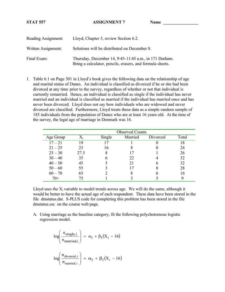
1. Table 6.1 on Page 301 in Lloyd’s book gives the following data on the relationship of age
and marital status of Danes. An individual is classified as divorced if he or she had been
divorced at any time prior to the survey, regardless of whether or not that individual is
currently remarried. Hence, an individual is classified as single if the individual has never
married and an individual is classified as married if the individual has married once and has
never been divorced. Lloyd does not say how individuals who are widowed and never
divorced are classified. Furthermore, Lloyd treats these data as a simple random sample of
185 individuals from the population of Danes who are at least 16 years old. At the time of
the survey, the legal age of marriage in Denmark was 16.
Age Group
17 – 21
21 – 25
25 – 30
30 – 40
40 – 50
50 – 60
60 – 70
70+
Xi
19
23
27.5
35
45
55
65
75
Single
17
16
8
6
5
3
2
1
Observed Counts
Married
Divorced
1
0
8
0
17
1
22
4
21
6
17
8
8
6
3
5
Total
18
24
26
32
32
28
16
9
Lloyd uses the Xi variable to model trends across age. We will do the same, although it
would be better to have the actual age of each respondent. These data have been stored in the
file dmstatus.dat. S-PLUS code for completing this problem has been stored in the file
dmstatus.ssc on the course web page.
A. Using marriage as the baseline category, fit the following polychotomous logistic
regression model.
 π single, i 
 = α1 + β1 (X i − 16)
log
 π married, i 


 π divorced , i 
 = α2 + β2 (X i − 16 )
log
 π married , i 


2
2
Report a value of a log-likelihood ratio G test, and its degrees of freedom and p-value,
for testing the fit of this model against the general alternate of eight different and
independent multinomial distributions for the eight age groups. Examine the plot of the
estimated curves against age. This plot also shows the observed proportions of
respondents in the three response categories at each level. Does this model appear to be
appropriate for the data?
B. Does the model
 π sin gle, i
log
 π married, i


 = α1 + β1(Xi − 16 ) + γ1(Xi − 16 )2


 πdivorced, i 
 = α2 + β 2 (X i − 16) + γ 2 (Xi − 16 )2
log
 π married, i 


appear to be appropriate for these data?
C. Does the model
 πsin gle , i 
 = α1 + β1 log(X i − 16 )
log
 π married , i 


 π divorced , i 
 = α2 + β2 log(Xi − 16)
log
 π married , i 


appear to be appropriate for these data?
D. Does the model
 πsin gle , i 
 = α1 + β1 log(X i − 16 ) + γ1 [log(X i − 16 )]2
log
 π married , i 


 π divorced , i 
 = α2 + β2 log(X i − 16 ) + γ 2 [log(Xi − 16)]2
log
 π married , i 


appear to fit these data?
3
E. Which of the models from parts A-D, if any, provides an adequate description of the
relationships between marital status and age in Denmark? Describe these relationships.
2. One alternative to searching for parametric curves to describe the Danish marital status data,
from Problem 1, is to fit non-parametric curves. In Section 5.2, Lloyd describes how the
generalized additive modeling (gam) function in S-PLUS can be used to do this. GAM
models have the form
link function = β0 +
K
∑ βj X ji +
j =1
∑ f j (X ji )
P
j= k + 1
where (X1i , ..., X Pi ) are the values of the P explanatory variables for the i-th case (or
respondent). The functions f j ( ) : j = k + 1, ..., P are not specified, they are estimated with
smoothing routines such as loess, kernel smoothers, or smoothing splines. Obviously, this
approach does not yield parametric formulas for curves, but the predict.gam command can be
used to compute a list of “smoothed” values at points on a grid that can be used to display the
“smoothed” curve. This can be helpful in detecting trends or patterns.
{
}
The S-PLUS code in the file dmstatus.ssc uses the gam ( ) function to fit the model
 πsin gle , i 
 = α1 + β1 log(X i − 16 ) + f1 X i − 16
log
 π married , i 


(
)
 π divorced , i 
 = α2 + β2 log(X i − 16) + f 2 X i − 16
log
 π married , i 


(
)
to the Danish marital status data from Problem 1. Examine the resulting plots. What do they
reveal? (Note that this approach may have performed better if the data file contained the
actual age of each respondent instead of only 8 unique age values.)
3. The data for this problem come from a randomized clinical trial involving treatment of
patients with squamous carcinoma (cancer) at various sites in the mouth and throat. Patients
who agreed to participate in the study were randomly assigned to one of two treatment
groups, radiation therapy alone or radiation therapy together with a chemotherapeutic agent.
The primary objective of this analysis is to compare the two treatments with respect to
patient survival at one year after treatment was initiated.
Although certain criteria had to be met for a patient to be eligible for this study, which
eliminated extremes in the extent of the disease, many factors are not controlled. The study
included measurement of many covariates that could be related to survival. Seven of those
variables are included in the data. The year that the patient entered the study is also recorded
on the data file.
4
The data are stored in the file oncology.dat. There is one line of data for each of the 195
patients examined in the study. The variables appear in the following order.
Columns
Variable
Codes
1-3
5
7
9
CASE
SEX
TREAT
GRADE
11-12
14
AGE
SITE
16
TSTAGE
18
NSTAGE
20−21
23
YEAR
STATUS
A 3 digit patient identification number
1 = male, 2 = female
1 = radiation only, 2 = radiation and chemotherapy
1 = well differentiated
2 = moderately differentiated
3 = poorly differentiated
age in years at start of treatment
1 = faucial arch
2 = tonsillar fossa
3 = posterior pillar
4 = pharyngeal tongue
5 = posterior wall
1 = primary tumor less than 2 cm. in diameter
2 = primary tumor between 2 cm. and 4 cm.
3 = primary tumor more than 4 cm. in diameter
4 = massive invasive tumor
0 = no clinical evidence of node metastases
1 = single positive node 3 cm. or less in diameter
2 = single positive node more than 3 cm. in diameter
3 = multiple positive nodes
Year patient started treatment (1978 through 1982)
0 = died within one year of beginning treatment
1 = survived for at least one year
The tumor state (TSTAGE) and node stage (NSTAGE) classifications provide an indication of
the prevalence of tumors at the primary site and neighboring lymph nodes. TSTAGE=1 refers
to a small isolated tumor at the primary site, whereas, TSTAGE=4 refers to a massive tumor
extending into the adjoining tissue. TSTAGE levels 2 and 3 refer to intermediate cases.
NSTATE=0 indicates no evidence of lymph node metastasis and NSTAGE values 1, 2, and 3
indicate increasing lymph node involvement. Patients with classifications (1,0), (1,1), (2,0), or
(2,1) for (TSTAGE, NSTAGE) were excluded from the study. The variable GRADE provides
an indication of the degree of differentiation of the tumor (the degree to which the tumor cells
resemble the host cells) from 1 (well differentiated) to 3 (poorly differentiated).
In addition to the primary question of whether the combined radiation and chemotherapy
treatment provides higher one year survival rates than the radiation treatment, it is of
considerable interest to determine the extent to which the covariates (SEX, GRADE, AGE,
SITE, TSTAGE, NSTATE, YEAR) are associated with one year survival rates.
Code for applying the SAS version of the CHAID algorithm is stored in the file oncology.sas
on the course web page. Code for applying the S-PLUS tree ( ) function to these data is
stored in the file oncology.ssc. Use this code to investigate associations between the covariates
and the one year survival rate. Under what circumstances, if any, do the one year survival rates
differ for the two treatments? Which treatment is better? How would you use these results to
help formulate a logistic regression model for predicting one year survival?