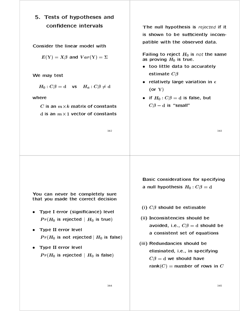
5. Tests of hypotheses and
con dence intervals
Consider the linear model with
E (Y) = X and V ar(Y) = We may test
H0 : C = d vs Ha : C 6= d
where
C is an m k matrix of constants
d is an m 1 vector of constants
The null hypothesis is rejected if it
is shown to be suÆciently incompatible with the observed data.
Failing to reject H0 is not the same
as proving H0 is true.
too little data to accurately
estimate C
relatively large variation in (or Y)
if H0 : C = d is false, but
C d is \small"
343
342
You can never be completely sure
that you made the correct decision
Type I error (signi cance) level
P r(H0 is rejected j H0 is true)
Type II error level
P r(H0 is not rejected j H0 is false)
Type II error level
P r(H0 is rejected j H0 is false)
344
Basic considerations for specifying
a null hypothesis H0 : C = d
(i) C should be estimable
(ii) Inconsistencies should be
avoided, i.e., C = d should be
a consistent set of equations
(iii) Redundancies should be
eliminated, i.e., in specifying
C = d we should have
rank(C ) = number of rows in C
345
Example 5.1 E ects model (from
Example 3.2)
Yij = + i + ij i = 1; 2; 3
j = 1; : : : ; ni
In this case
2
3 2
Y11
1
6 Y12 7 6 1
6
7 6
6 Y21 7 6 1
6
7 6
6 Y31 7 = 6 1
6
7 6
4 Y32 5 4 1
Y33
1
1
1
0
0
0
0
0
0
1
0
0
0
3
2
3
0 2 3 11
0 77 66 12 77
0 77 66 1 77+66 21 77
1 77 4 2 5 66 31 77
1 5 3 4 32 5
1
33
By de nition
E (Yij ) = + i is estimable.
We can test
H0 : + 1 = 60 seconds
against
HA : + 1 6= 60 seconds
(two-sided alternative)
Or we can test
H0 : + 1 = 60 seconds
against
HA : + 1 < 60 seconds
(one-sided alternative)
346
In this case
+
1
= cT
2
3
1
617
where c = 64 0 75
0
Note that this quantity is
estimable, e.g.,
cT = + 1 = E ((12 12 0 0 0 0)Y):
Then, any solution
yields the same value for cT b and it
is the unique blue for cT .
We will reject H0 : cT = 60 if
cT b = cT (X T 1X ) X T 1Y
b = (X T 1X ) X T 1Y
is too far away from 60.
to the generalized least squares estimating equations
X T 1X b = X T 1Y
347
348
Gauss-Markov Model
If Var(Y) = 2I , then any solution
b = (X T X ) X T Y
to the least squares estimating
equations
XT Xb = XT Y
yields the same value for
cT b is the unique blue for
cT b,
cT .
and
The di erence between mean
responses for two treatments
is estimable
1
3
= ( + 1) ( + 3)
1
1
1
1
1
= 2 2 0 3 3 3 E (Y)
and we can test
H0 : 1 3 = 0 vs. HA :
1
3
6= 0
If Var(Y) = 2I , the unique blue
for 1 3 = (0 1 0 1) = cT
is cT b for any b = (X T X ) X T Y
Reject H0 : 1 3 = cT = 0 if
cT b is too far from 0.
We will reject H0 : cT = 60 if
cT b = cT (X T X ) X T Y
is too far away from 60.
350
349
It would not be sensible to test
H0 : 1 = 3 vs. HA : 1 6= 3
because 1 = [0 1 0 0] = cT
is not estimable
Although E(Y1j ) = + 1, neither nor
has a clear interpretation.
Di erent solutions to the normal equations produce di erent values for
^ 1 = cT b = cT (X T X ) X T Y
1
To make a statement about 1, an
additional restriction must be imposed
on the parameters in the model to give
1 a precise meaning (pages 258-266).
351
In Example 3.2 (pages 155-161) we
found several solutions to the normal equations:
3
2
0 0 0 0 2 Y:: 3 2 0 3
6 0 1 0 0 7 6 Y 7 6 61 7
b = 664 0 02 1 0 775 64 Y12:: 75 = 64 71 75
1
69
0 0 0 31 Y3:
2
6
b = 13 64
1
1
1
0
1
2:5
1
0
1
1
4
0
32
3
2
0 Y::
0 77 66 Y1: 77 = 66
0 5 4 Y2: 5 4
0 Y3:
352
3
69
8 77
25
0
For
2
010
C=41 1 0
3
1
05
100 1
2
6
6
b = 66
4
2
6
1
6
1
6
1
6
1
6
1
2
1
6
1
6
0 11
0 0
1
3
0
3
2
2
3
Y::
0 777 66 Y1: 77 = 666
0 75 4 Y2: 5 4
Y3:
66:66 3
5:66 777
4:33 5
2:33
consider testing
2
1
3
1
3
H0 : C = 4 +
+
versus
2
3
2
5=4
3
3
60 5
70
3
3
60 5
70
HA : C 6= 4
353
In this case C is estimable, but
there is an inconsistency. If the null
hypothesis is true,
2
1
C =4 +
+
3
1
3
3
5=4
Then,
+ 1 = 60 and +
implies that
(
1
3
2
3
3
3
60 5
70
2
For
3
010 1
C=41 1 0 05
100 1
consider testing
2
1
H0 : C == 4 +
+
versus
= 70
2
) = ( + 1) ( + 3)
= 60 70 = 10
HA : C 6= 4
3
1
3
3
2
5=4
3
10
60 5
70
3
10
60 5
70
Such inconsistencies should be
avoided.
354
355
In this case C is estimable and
the equations speci ed by the null
hypothesis are consistent.
There is a redundancy
[1 1 0 0] = + 1 = 60
[1 0 0 1] = + 3 = 70
imply that
[0 1 0
The rows of C are not linearly independent, i.e., rank(C ) < number
of rows in C .
There are many equivalent ways to
remove a redundancy:
H0 : 11 10 00 10
1] = 1 3
= ( + 1) ( + 3)
= 60 70 = 10
H0 : 01 11 00
H0 : 01 10 00
H0 : 12 21 00
= 60
70
1 = 10
0
60
1 = 10
1
70
1 = 50
1
130
are all equivalent.
356
357
In each case:
The two rows of C are linearly
independent and
rank(C ) = 2
= number of rows in C
The two rows of C are a basis
for the same 2-dimensional
subspace of R4.
This is the 2-dimensional space
spanned by the rows of
2
3
010 1
C=41 1 0 05
100 1
358
We will only consider null
hypotheses of the form
H0 : C = d
where
rank(C ) = number of rows in C .
This leads to the following concept
of a \testable" hypothesis.
359
Defn 5.1: Consider a linear model
E (Y) = X where V ar(Y) = and
X is an n k matrix.
For an m k matrix of constants C
and an m 1 vector of constants d,
we will say that
H0 : C = d
is testable if
(i) C is estimable
(ii) rank(C ) = m
= number of rows in C
To test H0 : C = d
(i) Use the data to estimate C .
(ii) Reject H0 : C = d if the
estimate of C is to far away
from d.
Can the deviation of d from
the estimate of C be
attributed to random errors?
{ measurement error
{ sampling variation
Need a probability distribution for the estimate of C
Need a probability distribution for a test statistic
360
Normal Theory
Gauss-Markov Model
2
361
Result 5.1. (Results for the
Gauss-Markov model)
3
Y1
Y = 4 .. 5 N (X ; 2I )
Yn
For a testable null hypothesis
H0 : C = d
For any generalized inverse of
XT X,
b = (X T X ) X T Y
the OLS estimator for C ,
C b = C (X T X ) X T Y ;
has the following properties:
is a solution to the normal
equations
(i) Since C is estimable, C b
is invariant to the choice of
(X T X ) . (Result 3.10))
(X T X )b = X T Y :
362
363
(ii) Since C is estimable, C b is
the unique b.l.u.e. for C .
(Result 3.11)
(iii)
E (C b d) = C d
V ar(C b d) = V ar(C b)
= 2C (X T X ) C T
This follows from V ar(Y) = 2I ,
because
V ar(C b)
= V ar (C (X T X ) X T Y)
= C (X T X ) X T V ar (Y) X [(X T X ) ]T C T
= C (X T X ) X T ( 2I )X [(X T X ) ]T C T
= 2C (X T X ) X T X [(X T X ) ]T C T
Since C is estimable, C = AX for
some A (see Result 3.9 (i)) and
V ar(C b)
= 2AX (X T X ) X T X (X T X ) X T X T AT
= 2AX (X T X ) X T [X (X T X ) X T ]T AT
= 2AX (X T X ) X T AT
= 2C (X T X ) C T
365
364
(vi) The distribution of
SSH0 = (C b
(iv) C b d N (C d, C (X T X ) C T )
This follows from
2
Y N (X ; 2I );
property (iii) and Result 4.1.
d)T [C (X T X )
CT ]
(C b
d)
(C
d)
1
is given by
1 SS 2 (Æ2)
m
2 H
where m = rank(C ) and
0
Æ2 = 12 (C
d)T [C (X T X )
CT ]
1
This follows from Result 4.7 using
C b d N (C
(v) When H0 : C = d is true,
C b d N (0; 2C (X T X ) C T )
366
d; 2C (X T X ) C T )
A = 12 [C (X T X ) C T ] 1
= V ar(C b d)
= 2 C (X T X ) C T
Clearly, A = I is idempodent.
367
We also need the estimability of C
and
rank(C ) = m = number of rows in C
to ensure that C (X T X ) C T is
positive de nite and
(C (X T X ) C T ) 1 exists. Then,
Since C (X T X ) C T is positive
de nite, we have
Æ2
=
>
1
2 2
d)T [C (X T X )
(C
CT ]
1
(C
0
unless C
d = 0.
Hence Æ2 = 0 if and only if
H0 : C = d is true.
Consequently, from Result 4.7, we
have
d:f: = rank(A)
= rank(C (X T X ) C T )
=m
(vii) 1 SSH 2m if and
only if H0 : C = d is true.
2
0
369
368
Then,
To obtain an estimate of
V ar(C b d) = 2C (X T X ) C T
we need an estimate of 2.
Since E (Y) = X is estimable,
Y^ = X b = X (X T X ) X T Y = PX Y
SSresiduals = eT e
= YT (I PX )Y
is invariant to the choice of (X T X )
used to obtain PX = X (X T X ) X T
and b.
is the unique b.l.u.e. for X .
Consequently, the residual vector
e = Y Y^ = (I PX )Y
is invariant to the choice of (X T X )
used to obtain PX = X (X T X ) X:T
370
371
d)
Result (viii) is obtained by applying
Result 4.6 to
(viii) An unbiased estimator of 2 is
SSresidual = YT(I PX)Y
to obtain
where
E (YT (I PX )Y)
MSresiduals = SSnresiduals
k
=
tr((I PX )2I )
+ T X T (I PX )X
"
this is a zero matrix
k = rank(X) = rank(PX)
=
=
and
=
2tr(I PX )
2(tr(I ) tr(PX ))
2(n k)
where k = rank(X )= tr(PX ).
n k = rank(I PX)
This uses the assumption of a
Gauss-Markov model, but does not
use any normality assumption.
372
(ix) 1 SSresiduals 2n
2
k
To show this use the assumption
that Y N (X ; 2I ) and
apply Result 4.7 to
1
2
SSresiduals = YT
%
h
1
2
i
(I PX) Y
E (Y) = X = V ar(Y) = 2I = 373
-
this is A
The noncentrality parameter is
Æ2 = T A
= 12 T X T (I PX )X = 0
%
this is a matrix
of zeros
Clearly
A = 1 (I PX )2I = I PX
is idempotent.
2
374
375
(x) SSH and SSresiduals are
independently distributed.
0
To show this note that SSH
is a function of
Then, by Result 4.4, C b and e are
independent because
Cov(C b; e)
0
=
=
C b = C (X T X ) X T Y
=
and SSresiduals is a function of
=
e = (I X )Y
By Result 4.1,
C b = C (X T X ) X T Y
e
I PX
has a multivariate normal
distribution 2
because
Y N (X ; I ).
Cov(C (X T X ) X T Y; (I PX )Y)
C (X T X ) X T (V ar(Y))(I PX )T
C (X T X ) X T (2I )(I PX )
2C (X T X ) X T (I PX ) = 0
%
This is a matrix of
zeros since it is
the transpose of
(I PX )X = X X = 0
Consequently, SSH is independent
of SSresiduals, and it follows that
0
377
376
(xi)
SSH0
F = SS m2
residuals
(n k)2
SSH0
m
= SSresiduals
n k
Fm;n k(Æ2)
Perform the test by rejecting
H0 : C = d if
F > F(m;n k);
where is a speci ed signi cance
level (Type I error level) for the
test.
with noncentrality parameter
Æ2
=
1
2 (C
d)T [C (X T X )
CT ]
1
(C
d)
0
and Æ2 = 0 if and only if H0 : C = d
is true.
378
= P r frejectH0j H0 is trueg
379
Type I error level:
H0
residuals
This is the probability of incorrectly
rejecting a null hypothesis that is
true.
0.6
0.4
when H0 is true,
F = MSMS
has a central F distribution
with (m; n k) d.f.
0.8
j H0 is true
0.2
%
k;
0.0
= P r F > Fm;n
Central F Distribution with (4,20) df
f(x;n)
0
1
2
3
4
5
x
380
381
Type II error level:
= P rfType II errorg
= P rffail to reject H0 H0 is falseg
= P rfF < Fm;n
%
k;
H0 is falseg
when H0 is false;
F = MSMSH
residuals
has a noncentral F distribution
with (m; n k) d:f : and
noncentrality parameter Æ > 0:
0
382
Power of a test:
power = 1
= P rfF > Fm;n k; H0 is falseg
%
this determines
the value of
the noncentrality
parameter.
383
0.8
Central and Noncentral F Densities
with (5,20) df and noncentrality parameter = 1.5
0.6
Central
Central
FF
Central F
Noncentral F
f(x;v,w)
0.4
Noncentral
Noncentral
F(3)
F(3)
Noncentral
Noncentral
F(5)
F(5)
0.4
Noncentral
Noncentral
F(1)
F(1)
0.0
0.2
0.2
f(x;v,w)
0.6
0.8
Central and Noncentral
F Distributions with (4,20) df
1
2
3
4
5
0.0
0
x
0
1
2
3
4
5
x
384
385
0.6
0.6
0.8
Central and Noncentral F Densities
with (5,20) df and noncentrality parameter = 10
0.8
Central and Noncentral F Densities
with (5,20) df and noncentrality parameter = 3
Central F
Central F
0.4
0.2
0.0
0.2
0.4
f(x;v,w)
Noncentral F
0.0
f(x;v,w)
Noncentral F
0
1
2
3
4
5
0
x
1
2
3
4
5
x
386
387
Central and Noncentral F Densities
with (5,20) df and noncentrality parameter = 20
0.6
0.8
For a xed type I error level
(signi cance level) , the
power of the test increases as the
noncentrality parameter increases.
Central F
0.4
Æ2 =
1
T
T
T 1
2 (C d) [C (X X ) C ] (C
- size of
how much
0.2
f(x;v,w)
Noncentral F
the error the actual of the experiment
variance value of
(Note: the number
C
of observations
deviates
also a ects
from the
degrees of
hpothesized freedom.)
value d
0.0
0
1
2
3
4
d)
the design
5
x
389
388
Example 3.2 E ects of three diets
on blood coagulation times in rats.
Diet factor: Diet 1, Diet 2, Diet 3
Response: blood coagulation time
Model for a completely randomized
experiment with ni rats assigned to
the i-th diet.
Yij = + i + ij
Test the null hypothesis that the
mean blood coagulation time is the
same for all three diets
H0 : +
1
=+
2
=+
3
against the general alternative that
at least two diets have di erent
mean coagulation times
HA : (+ i) 6= (+ j ) for some i 6= j :
Equivalent ways to express the null
hypothesis are:
where
ij NID(0; 2)
for i = 1; 2; 3 and j = 1; 2; :::; ni.
H0 :
390
1
=
2
=
3
391
H0 : C = 00 10
= 00
= 00
0)T [C (X T X )
SSH0 = (C b
2
H0 : C = 00 10 01
Evaluate
3
1
1
2
3
6 7
0 6 17
1 4 25
=
3
1 66 1 77
1 4 25
MSH0 =
3
X n (Y
3
SSH0
2
on 3
SSresiduals = YT (I
MSresiduals =
The OLS estimator for C is
C b where b = (X T X ) X T Y
1
(C b
1 = 2 d:f :
PX )Y =
SSresiduals
X(n
3
i
on
n
XX
(Y
3
i
i=1 j =1
X(n
3
i
0
residuals
3
=1
1));
How many observations (in this
case rats) are needed? Suppose we
are willing to specify:
ij
Yi:)2
1) d:f :
i=1
1)
i=1
392
Reject H0 in favor of Ha if
F = MSH > F(2;Pi (ni
MS
0)
Y::)2
i i:
i=1
CT ]
393
For this particular alternative
2
3
6 7 0
1
0
1
:
5
1
C = 0 0 1 1 64 2 75 = 3
and the power of the F-test is
(i) = type I error level = .05
(ii) n1 = n2 = n3 = n
(iii) power .90 to detect
(iv) a speci c alternative
( + 1) ( + 3) = 0:5
( + 2) ( + 3) = n
power = Pr F(2;3n 3)(Æ2) > F(2;3n
394
395
3);:05
o
In this case,
where
1
:
5
Æ = 2
2
h
C (X T X ) C
= [:5 1]
0
0
T
i T 1 :5
h
C (X T X ) C T
%
i 1 :5 0
0
1
2
3n n
6
X T X = 64 nn n0
n 0
n n
2
0
0
0
6
(X T X ) = 64 00
0
and
Æ =
2
0
n
C (X T X ) C T
n rows of (1 0 1 0)
n rows of (1 0 0 1)
0 0 77
n 05
0 n
and a generalized inverse is
Then,
X has n rows of (1 1 0 0)
3
1
0
0
0
0 n
0 0 n
1
1
7
7
5
1
2
1
=n 1 2
[:5 1][C (X T X ) C T ]
1
= n2
396
3
:5
1
397
3):05
0.4
3)
n >F
(2;3n
2
0.2
0.0
:90 = power
= P r F(2;3n
Power
Choose n to achieve
0.6
0.8
1.0
Power versus Sample Size
F-test for equal means
0
10
20
30
40
50
Sample Size
398
For testing
# This file is stored in power.ssc
H0 : (+ 1) = (+ 2) = = (+ k)
against
#===========================================
n <- 2:50
d2 <- n/2
power <- 1 - pf(qf(.95,2,3*n-3),2,3*n-3,d2)
#
#
Unix users show insert the motif( )
function here to open a graphics window
HA : (+ 1) 6= (+ j )for somei 6= j
par(fin=c(7.5,8.5),cex=1.2,mex=1.5,lwd=4,
mar=c(5.1,4.1,4.1,2.1))
use
plot(c(0,50), c(0,1), type="n",
xlab="Sample Size",ylab="Power",
main="Power versus Sample Size\n
F-test for equal means")
lines(n, power, type="l",lty=1)
F = MSMSH0 F(k 1;Pki=1(ni
residuals
1))
(Æ2)
#============================================
400
399
where
with
Æ2 = 12
k
X
i=1
ni ( i
To obtain the formula for the noncentrality parameter, write the null
hypothesis as
H
0:0=C =
02
3 2
31 2 3
: )2
0
B
60
B
@64 .
0
k
X
: = i=1k
i=1
0
1
...
Use
ni i
X
1
0
0
0
ni
X
. 0
0
0
1
.
0
0
2
1
61
6
61
61
6
= 666 1.
6.
6 ..
6
4 ..
1
1
1
0
0
..
..
..
:
1
n
:
n
n
n
n
k
:
k
66 1
77C
5C
A 664 .2
:
k
03
0 77
0 77
0 77
0 77
.. 7
1 77
15
1
0 0
0
1
1
..
..
..
100
401
n1
n
77 66 0 ..
5 4 . ..
n
402
77
77
5
2
XT X
n: n1 n2 n1
n2
...
nk
nk
6 n1
6
= 66 n. 2
4.
nk
7
7
7
7
5
2
3
4 ..
7
7
7
7
7
5
0 0 0 0
6 0 n 1 0 0
6
1
(X T X ) = 666 0 0 n2 1 0
...
0 0 Then
=
=
1
0)T [C (X T X )
2 (C
k
1 X
n(
2 i=1 i
1
CT ]
nk 1
1
(C
:
Defn 5.2: Suppose Z N (0; 1)
is distributed independently of
W 2v , then the distribution
of
t = qZ
W
v
is called the student t-distribution
with v degrees of freedom.
0)
We will use the notation
t tv
:)2
404
403
# This code is stored in:
0.4
2 df
5 df
30 df
0.2
0.3
tden.ssc
#=================================================#
# t.density.plot()
#
# -----------------------#
# Input : degrees of freedom; it can be a vector. #
#
(e.g.) t.density.plot(c(2,5,7,30))
#
#
creates curves for df = 2,5,7,and 30 #
# Output: density plot of Student t distribution. #
# Note: Unix users must first use
motif()
#
#
to open a grpahics window before
#
#
using this function.
#
#================================================ #
Central t Densities
0.1
t.density.plot <- function(df)
{
x <- seq(-4,4,,100)
# draw x,y axis and title
0.0
f(x;df)
Æ2
Con dence intervals for
estimable functions of
3
-4
-2
0
2
plot(c(-4,4), c(0,.4), type="n",
xlab="x", ylab="f(x;df)",
main="Central t Densities")
4
x
for(i in 1:length(df)) {
lty.num <- 2*i-1
# specify the line types.
f.x <- dt(x,df[i])
# calculate density.
lines(x, f.x, type="l",lty=lty.num)
# draw.
}
405
406
For the normal-theory
Gauss-Markov model
Y N (X ; 2I )
and from Result 5.1.(iv) we have
for an estimable function, cT , that
the OLS estimator
# The following code creates a legend;
}
#
#
#
#
#
#
#
#
legend( x = rep(0.85,length(df)) ,
y = rep(.4,length(df)) ,
legend = paste(as.character(df),"df") ,
lty = seq(1,by=2,length=length(df)) ,
bty = "n")
cT b = cT (X T X ) X T Y
This function can be executed as follows.
Windows users should delete the motif( )
command.
follows a normal distribution, i.e.,
cT b N (cT ; 2cT (X T X ) c) :
motif( )
source("tden.spl")
par(fin=c(7,8),cex=1.2,mex=1.5,lwd=4)
t.density.plot(c(2,5,30))
It follows that
T
T
Z=q c b c
N (0; 1)
2
T
T
c (X X ) c
407
408
From Result 5.1.(ix), we have
1 = 1 YT (I P )Y
X
2
2
2
(n
First note that
k)
where k = rank(X ).
Using the same argument that we
used to derive Result 5.1.(x), we
can show that cT1b is distributed independently of SSE.
cT b
(I PX )Y =
T T
c (X X )
XT Y
(I PX )
has a joint normal distribution
under the normal-theory GaussMarkov model. (From Result 4.1)
2
409
410
Also
Cov(cT b; (I PX )Y)
= (cT (X T X ) X T )(2I )(I PX )
= 2cT (X T X ) X T (I PX )
=0
"
this is a matrix of zeros
Then,
t= r Z
SSE
2(n
=
=
Consequently, (by Result 4.4)
cT b is distributed independently
of e = (I PX )Y
which imples that
cT b is distributed
independently
of SSE = eT e.
q
k)
cT b cT
2cT (X T X ) c
r
SSE
2(n
q
k)
cT b cT
t(n k)
SSE cT (X T X ) c
(n k)
%
SSE
n k
is the MSE
411
412
It follows that
Central t Density
( 5 degrees of freedom )
=
Pr
=
Pr
(
t(n
k); =2
t(n
cT b
cT b + t n
0.2
(
T
cT
c b
pMSE
c
T
q
tn
c
(
(XTX)
T
T
k); =2 MSE c (X X) c
)
k); =2
cT
q
T
T
k); =2 MSE c (X X) c
0.1
and a (1 ) 100% con dence
interval for cT is
0.0
f(x;df)
0.3
0.4
1
-4
-2
0
2
cT b
4
x
t(n k); =2 MSE cT(XTX) c ;
cT b + t
413
q
(n
k); =2
q
MSE c (X X) c
T
T
414
For brevity we will also write
cT b t(n
where
k); =2 ScT b
Con dence interval for 2
q
ScT b = MSE cT(XTX) c
For the normal-theory GaussMarkov model with Y N (X ; 2I )
we have shown that
For the normal-theory
Gauss-Markov model with
Y N (X ; 2I ); the interval
cT b t(n
SSE = YT (I PX )Y 2
2
k); =2ScT b
(n
2
k)
is the shortest random interval with
probability (1 ) of containing cT .
416
415
Then,
1
=
n
P r 2(n k);1 =2 SSE
2 (n k); =2
=(
P r 2 SSE
(n k);
=2
2 (n
SSE
;
k) 1
)
o
The resulting (1 ) 100% con dence interval for 2 is
0
@
SSE
2
(n k);
=2
;
1
SSE
2
(n k);1
=2
A
=2
417
418
0.0
0.04
f(x;df)
0.08
0.12
Central Chi-Square Density
0
5
10
15
20
25
30
x
419