Lecture 5: Systems of Equations
1.
(SUR) So, you’ve got a model with more than one equation: eg, consumer demand is
about modelling how all expenditure shares vary with prices, expenditure and
demographic characteristics.
a.
Yi j = X i j β j + ε i j , j = 1,..., M , i = 1,..., N .
i.
i=1,..,N indexes people, and j=1,..,M indexes equations. Note that the X’s
can differ across equations, as well as, of course, the parameters β .
We will assume the normal things about the error terms: mean zero for
each equation, homoskedastic for each equation.
We will allow for cross-equation correlations in the error terms, but no
correlations across people i.
j
ii.
iii.
ε i = [ε i1 ,..., ε iM ]'
(1)
b.
c.
E [ ε i ] = 0 M ∀i ,
E [ε i'ε i ] = Σ ∀i , E [ε i'ε j ] = 0 ∀i ≠ j
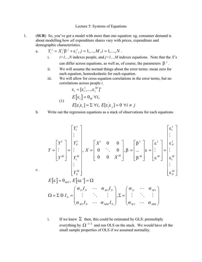
Write out the regression equations as a stack of observations for each equations
Y11 
ε11 
 
 
M 
M 
Y 1  YN1 
X1 0
β 1 
ε 1  ε 1N 
0 
   




   
Y = M  = M  , X =  0 O 0  , β = ...  ε = M  = M 
Y M  Y1M 
 0 0 XM
β M 
ε M  ε1M 
   




   
M 
M 
 M
 M
YN 
ε N 
E [ε ] = 0 MN , E [εε '] = Ω
 σ 11 I N
Ω = Σ ⊗ I N =  M
σ I
 M1 N
i.
If we knew
Σ
L σ M 1I N 
 σ 11 L σ M 1 
O
M  , Σ =  M
O
M 
σ

L σ MM I N 
 M 1 L σ MM 
then, this could be estimated by GLS: premultiply
everything by Ω −1/ 2 and run OLS on the stack. We would have all the
small sample properties of OLS if we assumed normality.
d.
Σ , then we could find a consistent estimate of it,
In contrast, if we didn’t know
µ , and then premultiply everything by Ω
µ
construct Ω
, and run OLS on the
stack. This is called feasible GLS (FGLS), and we can use only asymptotics
(though we don’t need to assume normality).
What is a consistent estimator for Ω ? How about do OLS on the stack, collect
−1/ 2
e.
the big vector of sample errors e =  e '... e '  ' (which is a vector of length
MN—N errors in each of M equations), and then calculate
1
M
Ω = {ω jk }, ω jk = E [ε jε k ],
{ }
µ= ω
µ jk , ω
µ jk = 1
Ω
N
N
∑e e
i =1
i
j k
i
f.
This FGLS strategy is called “seemingly unrelated regression” (SUR) because the
only connection across equations is in the disturbance terms—they are otherwise
seemingly unrelated.
g.
Cool thing: If X
j
= X K ∀j , k , then FGLS is identical to eq-by-eq OLS.