Mixture Modeling of the Distribution of p Wild-type vs. Myostatin Knockout Mice
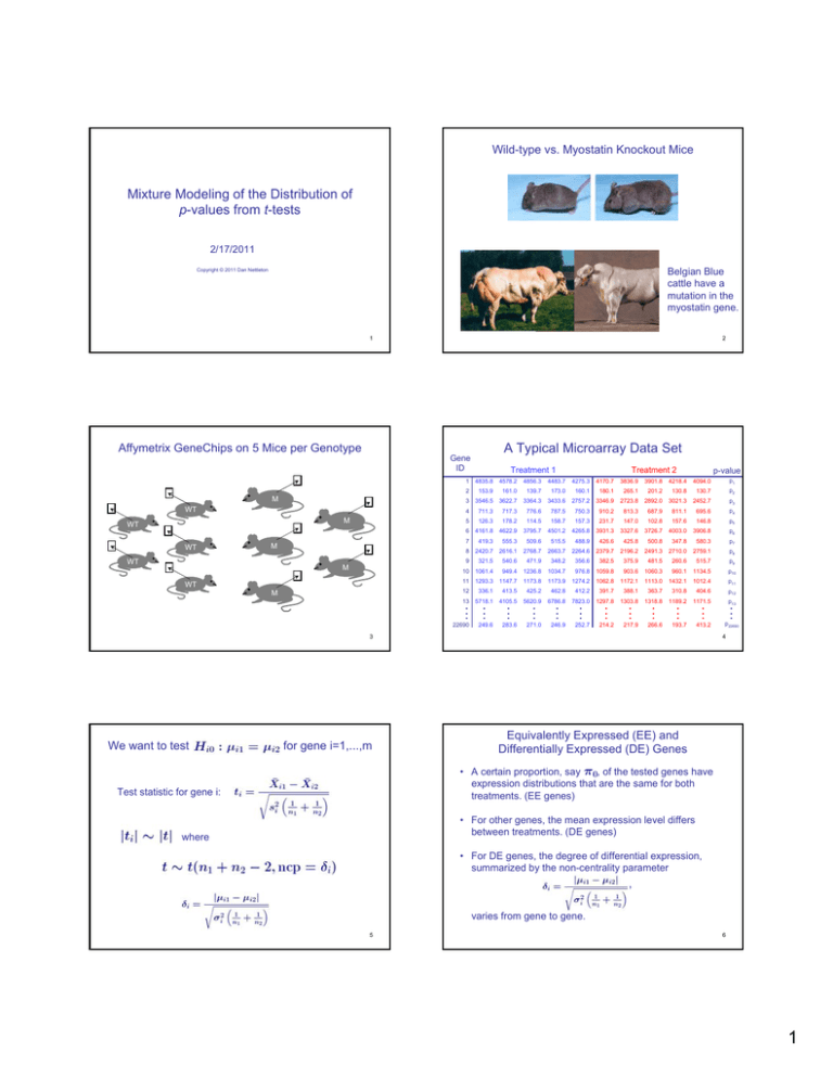
advertisement
Wild-type vs. Myostatin Knockout Mice Mixture Modeling of the Distribution of p-values from t-tests 2/17/2011 Belgian Blue cattle have a mutation in the myostatin gene. Copyright © 2011 Dan Nettleton 1 Affymetrix GeneChips on 5 Mice per Genotype WT M WT M WT M WT A Typical Microarray Data Set Gene ID M WT 2 Treatment 2 p-value 4835.8 4578.2 4856.3 4483.7 4275.3 4170.7 3836.9 3901.8 4218.4 4094.0 p1 2 153.9 161.0 139.7 173.0 160.1 180.1 265.1 201.2 130.8 130.7 p2 3 3546.5 3622.7 3364.3 3433.6 2757.2 3346.9 2723.8 2892.0 3021.3 2452.7 p3 4 711.3 717.3 776.6 787.5 750.3 910.2 813.3 687.9 811.1 695.6 p4 5 126.3 178.2 114.5 158.7 157.3 231.7 147.0 102.8 157.6 146.8 p5 6 4161.8 4622.9 3795.7 4501.2 4265.8 3931.3 3327.6 3726.7 4003.0 3906.8 p6 7 419.3 555.3 509.6 515.5 488.9 426.6 425.8 500.8 347.8 580.3 p7 8 2420.7 2616.1 2768.7 2663.7 2264.6 2379.7 2196.2 2491.3 2710.0 2759.1 p8 9 321.5 540.6 471.9 348.2 356.6 382.5 375.9 481.5 260.6 515.7 p9 10 1061.4 949.4 1236.8 1034.7 976.8 1059.8 903.6 1060.3 960.1 1134.5 p10 11 M Treatment 1 1 1012.4 p11 12 336.1 413.5 425.2 462.8 412.2 391.7 388.1 363.7 310.8 404.6 p12 13 .. . 5718.1 1293.3 193.7 .. . p13 266.6 .. . 1171.5 217.9 .. . 1189.2 214.2 .. . 1318.8 252.7 .. . 1303.8 246.9 .. . 1297.8 271.0 .. . 7823.0 283.6 .. . 6786.8 249.6 .. . 5620.9 22690 .. . 4105.5 1147.7 1173.8 1173.9 1274.2 1062.8 1172.1 1113.0 1432.1 413.2 p22690 3 We want to test for gene i=1,...,m .. . 4 Equivalently Expressed (EE) and Differentially Expressed (DE) Genes • A certain proportion, say , of the tested genes have expression distributions that are the same for both treatments. (EE genes) Test statistic for gene i: • For other genes, the mean expression level differs between treatments. (DE genes) where • For DE genes, the degree of differential expression, summarized by the non-centrality parameter , varies from gene to gene. 5 6 1 Conditional Distribution Function of the p-value Given the Non-Centrality Parameter Objectives • Estimate = proportion of non-centrality parameters that are zero (i.e., proportion of genes that are EE) • Estimate = density that approximates the true distribution of nonzero non-centrality parameters. • Estimate false discovery rates (FDR) • Estimate falsely interesting discovery rates (FIDR) • Perform power and sample size calculations for future experiments 7 Conditional Density of the p-value Given the Non-Centrality Parameter 8 Conditional Densities of p-values Given . = 0.5 1.0 1.5 2.0 p 9 10 Histogram of p-values from Two-Sample t-Tests The Marginal Distribution of the t-test p-value Number of Genes Suppose that each non-centrality parameter is 0 with probability and a draw from a continuous distribution with probability . Then the marginal density of the t-test p-value is given by . p-value 11 12 2 Approximate g with a Linear Spline Function where The B-Splines are B-splines normalized to be densities and . 13 fgf B-Splines Weighted δ 14 fgf Estimate of g Linear Spline 15 fgf B-Splines Weighted δ δ δ 16 fgf Estimate of g Linear Spline 17 δ 18 3 Approximating the Marginal Density of p-values p-value 19 p-value 20 p-value 21 p-value 22 p-value 23 24 4 p-value p-value 25 26 We seek a convex combination of the z functions that fits our empirical p-value distribution well. p-value 27 Bin p-values into 2000 Bins 28 Find fgf minimizes that Number of Histogram Bins (e.g., 2000) Observed Density Height for ith Bin Weight Assigned to ith Bin Semiparametric Approximation of Density Height for the ith Bin Smoothing Parameter Penalty for lack of smoothness in g Solved via quadratic programming. 29 30 5 Solution to the penalized least squares problem yields a convex combination of z functions as a density estimate. Two-Sample t-test p-values with Estimated Density 31 Two-Sample t-test p-values with Estimated Density 32 Note that the similarity of z1 and z2. The “compromise estimator” combines the portion of the density due to null p-values with the portion of the density due to “near null” p-values. 33 Two-Sample t-test p-values with Estimated Density 34 Estimated Density of Nonzero Non-Centrality Parameters 0.750 0.450 0.316 35 36 6 Histogram of 10000 p-values with Estimated Distribution True and Estimated NCP Densities g(δ)=gamma(6,3) m = 10000 B-spline estimate π0 = 0.85 g(δ)=gamma(6,3) 37 Density m0 = 8500 δ 38 Histogram of 10000 p-values with Estimated Distribution Parameter Estimates m = 10000 m0 = 7500 π0 = 0.75 g(δ)=gamma(2,2) 39 True and Estimated NCP Densities 40 Parameter Estimates Density g(δ)=gamma(2,2) B-spline estimate δ 41 42 7 Histogram of 10000 p-values with Estimated Distribution True and Estimated NCP Densities g(δ)=gamma(1,1.5) m = 10000 π0 = 0.70 g(δ)=gamma(1,1.5) 43 Density m0 = 7000 B-spline estimate δ 44 Histogram of 10000 p-values with Estimated Distribution Parameter Estimates m = 10000 m0 = 9000 π0 = 0.90 g(δ)=gamma(6,3) 45 True and Estimated NCP Densities 46 Parameter Estimates Density g(δ)=gamma(6,3) B-spline estimate δ 47 48 8 Other Estimators of . The Compromise Estimator There are many! Some examples include... Lowest Slope: Schweder and Spjotvoll (1982), Hochberg and Benjamini (1990), Benjamini and Hochberg (2000). Mixture of Uniform and Beta: Allison et al. (2002), Pounds and Morris (2003). λ Threshold: Storey (2002), Storey and Tibshirani (2003) In this case the compromise estimator is 0.8607 compared to = 0.8386 and = 0.9. 49 Other Estimators of Convex Density Estimation: Langaas, Ferkingstad, Lindqvist (2005) Histogram Based Estimation: Mosig et al. (2001), Nettleton et al. (2006) Moment Based Estimator: Lai (2007) 50 Myostatin p-values with Estimated Density for the Myostatin Data density uniform-beta mixture: 0.7506 λ-estimator: 0.7583 convex estimator: 0.7529 histogram estimator: 0.7515 0.750 0.450 0.316 p-value 51 Some Simulation Results Other Quantities of Interest 0.95 0.95 0.95 0.70 0.70 0.70 near medium far near medium far 0.0251 0.0276 0.0348 0.0145 0.0124 0.0148 0.0346 0.0066 0.0269 0.0121 0.0503 0.1519 0.0492 0.1485 0.1035 0.0748 0.0268 0.0767 0.0732 0.0187 0.0458 0.0214 RMSE -0.0286 -0.0063 -0.0703 -0.0233 -0.0014 0.1517 0.0743 0.0166 -0.0221 0.0367 0.0158 -0.0169 -0.0020 0.1476 0.0749 0.0167 BIAS compromise 0.0206 convex 0.0238 0.0001 -0.0228 0.0266 0.0123 compromise 0.0076 0.0007 convex 0.0208 0.0089 52 Posterior Probability of Differential Expression PPDE(p) = P(DE|p-value=p) “convex” is the estimator of Langaas et al. (2005) JRSSB 67, 555–572 53 False Discovery Rate FDR(c) = P(EE|p≤c) True Positive Rate TPR(c) = P(DE|p≤c) = 1 – FDR(c) True Negative Rate TNR(c) = P(EE|p>c) Expected Discovery Rate EDR(c) = P(p≤c|DE) Gadbury et al. (2004). Stat. Meth. in Med. Res. 13, 325-338 discuss last three quantities in power and sample size context. 54 9 Approximation for EDR Approximation for FDR 55 Power-Sample Size Calculations 56 Relationship between New NCP and Old NCP • If we have estimates of π0 and g(δ) from a previous experiment, we can examine how our ability to discover differentially expressed genes will vary with sample size. • Suppose the within-treatment sample sizes for a new experiment differ from the previous experiment by a factor of . • If denotes the NCP for a gene in the previous experiment, then the NCP for the same gene in the new experiment will be . • We can see how quantities of interest very with to guide samples size selection in the new experiment. 57 58 Power-Sample Size Calculations Approximate EDR for the New Experiment EDR degrees of freedom change to reflect the larger sample size replaces δ in the calculation for the previous experiment 59 TPR TNR p-value threshold for significance 60 10 “Interesting Discovery” Rates Main Reference Ruppert, D., Nettleton, D., Hwang, J.T.G. (2007). Exploring the information in p-values for the analysis and planning of multiple-test experiments. Biometrics. 63 483-495. researcher-determined threshold that defines “interesting discovery” 61 62 11
