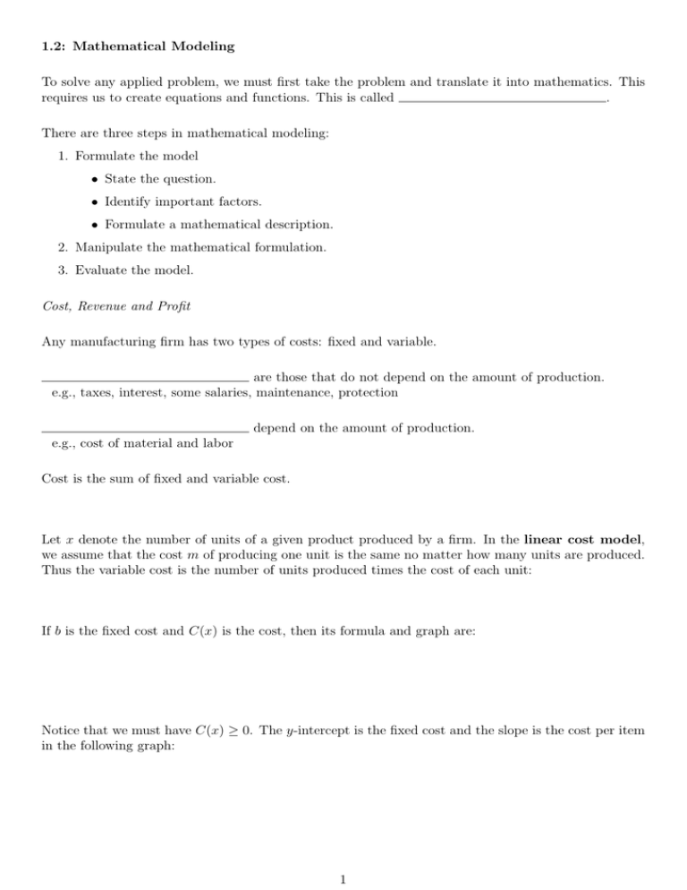
1.2: Mathematical Modeling
To solve any applied problem, we must first take the problem and translate it into mathematics. This
requires us to create equations and functions. This is called
.
There are three steps in mathematical modeling:
1. Formulate the model
• State the question.
• Identify important factors.
• Formulate a mathematical description.
2. Manipulate the mathematical formulation.
3. Evaluate the model.
Cost, Revenue and Profit
Any manufacturing firm has two types of costs: fixed and variable.
are those that do not depend on the amount of production.
e.g., taxes, interest, some salaries, maintenance, protection
depend on the amount of production.
e.g., cost of material and labor
Cost is the sum of fixed and variable cost.
Let x denote the number of units of a given product produced by a firm. In the linear cost model,
we assume that the cost m of producing one unit is the same no matter how many units are produced.
Thus the variable cost is the number of units produced times the cost of each unit:
If b is the fixed cost and C(x) is the cost, then its formula and graph are:
Notice that we must have C(x) ≥ 0. The y-intercept is the fixed cost and the slope is the cost per item
in the following graph:
1
In the linear revenue model, we assume that the price p of a unit sold by a firm is the same no
matter how many units are sold. Thus, the revenue is the price per unit times the number of units
sold. Let x be the number of units sold. (For convenience, we assume the number of units sold equals
the number of units produced.) Then, if we denote the revenue by R(x), then its formula and graph
are:
Notice that we must have R(x) ≥ 0. The line goes through (0, 0) because nothing sold results in no
revenue. The slope is the price per unit.
Regardless of whether our models of cost and revenue are linear or not,
P is always revenue less cost. Thus
Recall that both C(x) and R(x) must be nonnegative functions. However, profit P (x) can be positive
or negative. Negative profits are called
.
Example 1. (Tomastik) In 1996, Rogers and Akridge of Purdue University studied fertilizer plants in
Indiana. For a typical small-sized plant, they estimated fixed costs at $243,854 and estimated that it
costs $215.73 to produce each ton of fertilizer. The plant sells its fertilizer output at $264.82 per ton.
Find the cost, revenue, and profit equations.
The value of x at which the profit is zero is called the
even quantity is the value of x at which cost equals revenue.
. The break-
Example 2. Find the break-even quantity for the previous example. Round to two decimal places.
2
Supply and Demand
Assume that x is the number of units produced and sold by the entire industry during a given period
of time and that p = −cx + d, c > 0, is the price of one unit if x units are sold; that is, p = −cx + d
and the
is the price of the xth unit sold. We call p = −cx + d the
. Estimating the demand curve is a fundamental problem
graph the
for the management of any comany or business.
Note that the demand curve is typically decreasing.
Example 3. When the price for an item is set at $17, consumers are willing to buy 21 items. When the
price is set at $29, no consumer is willing to buy the item. Find the linear demand equation, p = D(x).
p = p(x) gives the price p necessary for suppliers to make availThe
.
able x units to the market. The graph of this equation is called the
A reasonable supply curve increases because the suppliers of any product naturally want to sell more
if the price is higher.
Example 4. The producer is not willing to sell any items if the price is set at $6. However, the producer
will supply 11 items when the price is $9. Find the linear supply equation, p = S(x).
3
The best-known law of economics is the law of supply and demand. The point where the supply curve
. The x-coordinate of the
intersects the demand curve is called the
equilibrium point is called the
and the p-coordinate is called the
.
2
Example 5. Suppose the price of an item is given by p = − x + 28 when x items are demanded.
3
2
Further, manufacturers are willing to sell x items at the price p = x + 7
5
a) What is the surplus or shortage if the price is set at $16?
b) What is the equilibrium quantity? What is the equilibrium price?
Example 6. (Tomastic, #27) Many assets, such as machines or buildings, have a finite useful life
and further more depreciate in value from year to year. For purposes of determining profits and taxes,
various methods of depreciation can be used. In straight-line depreciation we assume that the value
V of the asset is given by a linear equation in time t, say, V = mt + b. The slope m must be negative,
since the value of the asset decreases over time. Consider a new machine that costs $40,000 and has a
useful life of nine years and a scrap value of $4000. Using straight-line depreciation, find the equation
for the value V in terms of t, where t is in years. Find the value after one year and after five years.
4
Quadratic Mathematical Models
A quadratic is a polynomial function of degree 2:
function can be placed in standard form
the vertex and can be found by using the formulas
. Every quadratic
. The point (h, k) is called
We will now consider quadratic mathematical models of revenue and profit. If the number of units of
a product sold by an industry is to increase significantly, then the price per unit will most likely need
to decrease (by supply and demand). Therefore, if the demand equation for an entire industry is the
linear demand equation p = −cx + d with c > 0, then the revenue is:
This is a quadratic model!
2
Example 7. Suppose that price of an item is given by p = − x + 28 when x items are demanded.
3
a) Find the revenue function.
b) When is the revenue maximized?
5