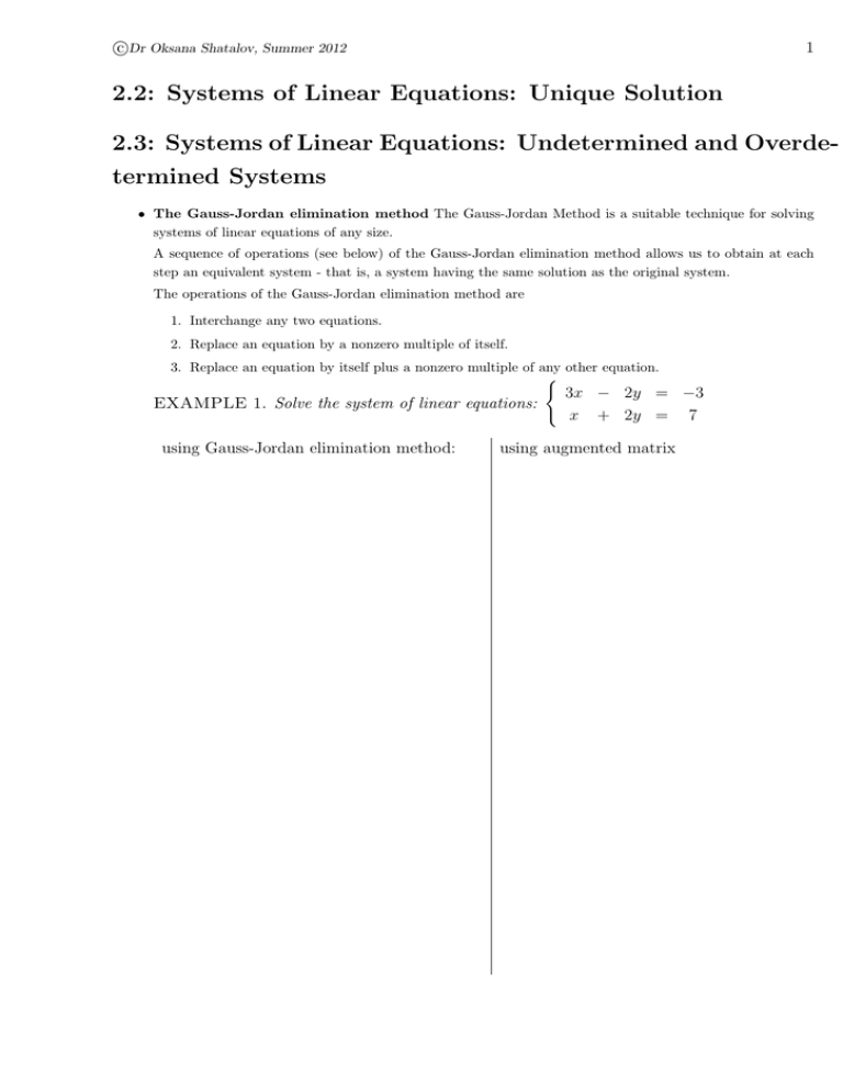
c Dr Oksana Shatalov, Summer 2012
1
2.2: Systems of Linear Equations: Unique Solution
2.3: Systems of Linear Equations: Undetermined and Overdetermined Systems
• The Gauss-Jordan elimination method The Gauss-Jordan Method is a suitable technique for solving
systems of linear equations of any size.
A sequence of operations (see below) of the Gauss-Jordan elimination method allows us to obtain at each
step an equivalent system - that is, a system having the same solution as the original system.
The operations of the Gauss-Jordan elimination method are
1. Interchange any two equations.
2. Replace an equation by a nonzero multiple of itself.
3. Replace an equation by itself plus a nonzero multiple of any other equation.
(
EXAMPLE 1. Solve the system of linear equations:
using Gauss-Jordan elimination method:
3x − 2y = −3
x + 2y = 7
using augmented matrix
c Dr Oksana Shatalov, Summer 2012
2
• Augmented Matrices
An augmented matrix that is formed by combining the coefficient matrix and the constant
matrix as shown in the next example.
EXAMPLE 2. Find the initial augmented matrix for the system of linear equations below:
(
3x1 + 12x2 = 20
(a)
2x2 = x1 +7


 3x − 2y + 5z = 100
(b)
x + z = 7


y − z = 11


 x = 1
(c)
y = 12


z = 5
The goal of the Gauss-Jordan Elimination Method is to get the augmented matrix into
Row-Reduced Echelon Form (rref).
Row-Reduced Echelon Form of Matrix (note that all rules apply to the coefficient part only.):
(I) The 1st nonzero entry in each row is a 1, called the leading 1.
(II) The leading 1 in a lower row must lie to the right of the leading 1 in a upper row.
(III) A row made entirely of zeros lies below any other row.
(IV) A column containing a leading 1 must be a unit column, that is, all other entries in
the column are zeros.
EXAMPLE

1 0

(a) 0 1
0 0

1

(d)  0
0

3
0
0
3. Indicate whether the


1
0 2 12
 0


3 0 -5  (b) 
 0
0 0 11
0

0 0

4 1 
0 0

1 0 0 15


(g)  0 0 1 1 
0 0 1 -10

matrix
0 0
0 0
1 7
0 0
1 0 0

(e)  0 1 0
0 0 1

is in row reduced form:


2 12
1 3 0
0 11 


 (c)  0 0 1
0 11 
0 0 0
0 0

5

6 
-11

1 0 0 15


(h)  0 1 0 1 
0 0 1 -10

1

(f ) 0
0
0
0
1

0

5 
1

0 0

1 22 
0 11
c Dr Oksana Shatalov, Summer 2012
3
To put a matrix in Row Reduced Form, there are three valid Row Operations:
1. Interchange any two rows (Ri ↔ Rj ).
2. Replace any row by a nonzero constant multiple of itself (cRi ).
3. Replace any row by the sum of that row and a constant multiple of any other row
(Ri + cRj ).
– The process in which a column transforms into a unit column is called pivoting.
– How to pivot:
1. Use ROW OPERATIONS to convert the circled pivot element into a 1.
2. Use ROW OPERATIONS to convert the other elements in the column into 0s.
The Gauss-Jordan method is to use pivot operations to work column by column until the
matrix is in reduced form. The solution(s) can then be reached from the corresponding
system.
EXAMPLE 4. Solve:
2x + 4y + 2z = −4
3x + 8y − z = −18
2x + y + 5z = 8


2 4 2

 3 8 -1
2 1 5

-4
1
 R1 ↔ 2 R1 
-18 
 3
−→
8
2



-2
1 2
1
 R2 ↔ 2 R2 
-12 
 0 1
−→
0 -3

1 2

 0 2

1
-4
1 0 5

 0 1 -2
0 0 -3

10

-6 
-6
8
1
-1
5

1
 R2 − 3R1 
-18 

−→
8
2

1 -2

-2 -6 
3 12

−→
2
1
-2
1
5
8
1 0

 0 1
0 -3
 R3 − 2R1 


−→

5 10

-2 -6 
3 12



1 0 5 10
1 0 0 0




−→
−→
 0 1 -2 -6 
 0 1 -2 -6 
0 0 1 2
0 0 1 2


1 0 0 0


−→
(x, y, z) = (0, −2, 2)
 0 1 0 -2 
0 0 1 2


−→

−→
c Dr Oksana Shatalov, Summer 2012
To put an augmented matrix into row-reduced form we can use calculator:
1. Enter the augmented matrix into your calculator.
2. Go to your home screen.
3. Hit 2nd x−1 , cursor right to MATH, and select B:rref.
4. Call the matrix you want to reduce and hit ENTER .
Now you can simply read off the solutions to your original system of equations.
EXAMPLE 5. Solve the system of Example 4 using your calculator.
EXAMPLE 6. Solve the system of linear equations:
(a)
2x + 11y = 70
5x − 2y = 25
x − 4y = 9
(b) 3y − 2x = 8
2x + 4y = 6
x + y + z = 1
(c) x + 5y + 5z = −1
3x − y − z = 4
4
c Dr Oksana Shatalov, Summer 2012
5
x + 2y + z = −2
EXAMPLE 7. (a) Solve 2x + 3y + z = −1
3x + 5y + 2z = −3

1 0 -1 4

Solution: The resulting rref matrix is  0 1 1 -3
0 0 0 0
There is no unique solution. We have a situation with



infinite solutions.
How can we express the solutions in a helpful way?
First, translate the rows back into equations:
Then solve for all other variables in terms of one of them in order to define a ”pattern”
for the infinite solutions.
– We can let the parameter t represent the z value (then x and y represent so called
basic variables)
and get the pattern:
(b) Use the general pattern for the solutions, (4+t,-3-t,t), to find the missing portions of these
specific solutions:
(1) (
,
, 10)
(2) (
,
, 0)
(3) (55,
,
)
c Dr Oksana Shatalov, Summer 2012
EXAMPLE 8. Solve:
x1 + 3x2 − x3
2x1 + 4x2 −
− 3x4
2x4
6
= 7
= 10
EXAMPLE 9. A chemical manufacturer wants to lease a fleet of 24 railroad tank cars with a combined carrying
capacity of 520,000 gallons. Tank cars with three different carrying capacities are available: 8,000 gallons, 16,000
gallons, and 24,000 gallons. How many of each type of tank car should be leased?
c Dr Oksana Shatalov, Summer 2012
7
EXAMPLE 10. A company wants to purchase 25 trucks with a combined capacity of 28, 000 ft3 . Three different
types of trucks are available: a 10-foot truck with a capacity of 350 ft3 , a 14-foot truck with a capacity of 7000 ft3 ,
and a 24-foot truck with a capacity of 1400 ft3 . How many of each type of truck should the company purchase?
c Dr Oksana Shatalov, Summer 2012
8
Useful Remark:

 
1 0 0 *
1 0

 
• The system has exactly one solution:  0 1 0 * ,  0 1
0 0 1 *
0 0


1 0 * *


• No solution:  0 1 * * , where a is a non zero constant.
0 0 0 a


"
#
1 0 * *
1 * 0 *


• Infinitely many solutions:  0 1 * * ,
0 0 1 *
0 0 0 0

*

* 
0