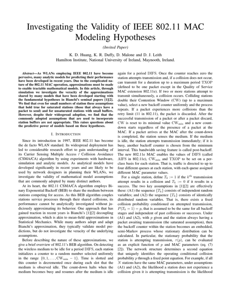
Investigating the Validity of IEEE 802.11 MAC
Modeling Hypotheses
(Invited Paper)
K. D. Huang, K. R. Duffy, D. Malone and D. J. Leith
Hamilton Institute, National University of Ireland, Maynooth, Ireland.
Abstract—As WLANs employing IEEE 802.11 have become
pervasive, many analytic models for predicting their performance
have been developed in recent years. Due to the complicated nature of the 802.11 MAC operation, approximations must be made
to enable tractable mathematical models. In this article, through
simulation we investigate the veracity of the approximations
shared by many models that have been developed starting with
the fundamental hypotheses in Bianchi’s seminal papers [1][2].
We find that even for small numbers of station these assumptions
that hold true for saturated stations (those that always have a
packet to send) and for unsaturated stations with small buffers.
However, despite their widespread adoption, we find that the
commonly adopted assumptions that are used to incorporate
station buffers are not appropriate. This raises questions about
the predictive power of models based on these hypotheses.
I. I NTRODUCTION
Since its introduction in 1997, IEEE 802.11 has become
the de facto WLAN standard. Its widespread deployment has
led to considerable research effort to gain understanding of
its Carrier Sensing Multiple Access / Collision Avoidance
(CSMA/CA) algorithm by using experiments with hardware,
simulation and analytic models. As analytical models have
developed significantly in recent years and are likely to be
used by network designers in planning their WLANs, we
investigate the validity of mathematical model assumptions
that are commonly adopted by many distinct authors.
At its heart, the 802.11 CSMA/CA algorithm employs Binary Exponential Backoff (BEB) to share the medium between
stations competing for access. As this BEB algorithm couples
stations service processes through their shared collisions, its
performance cannot be analytically investigated without judiciously approximating its behavior. One approach that has
gained traction in recent years is Bianchi’s [1][2] decoupling
approximation, which is akin to mean-field approximations in
Statistical Mechanics. While many authors adopt and adapt
Bianchi’s approximation, they typically validate model predictions, but do not investigate the veracity of the underlying
assumptions.
Before describing the nature of these approximations, we
give a brief overview of 802.11’s BEB algorithm. On detecting
the wireless medium to be idle for a period DIFS, each station
initializes a counter to a random number selected uniformly
in the range {0, 1, . . . , CWmin − 1}. Time is slotted and
this counter is decremented once during each slot that the
medium is observed idle. The count-down halts when the
medium becomes busy and resumes after the medium is idle
again for a period DIFS. Once the counter reaches zero the
station attempts transmission and, if a collision does not occur,
can transmit for a duration up to a maximum period TXOP
(defined to be one packet except in the Quality of Service
MAC extension 802.11e). If two or more stations attempt to
transmit simultaneously, a collision occurs. Colliding stations
double their Contention Window (CW) (up to a maximum
value), select a new backoff counter uniformly and the process
repeats. If a packet experiences more collisions than the
retry limit (11 in 802.11), the packet is discarded. After the
successful transmission of a packet or after a packet discard,
CW is reset to its minimal value CWmin and a new countdown starts regardless of the presence of a packet at the
MAC. If a packet arrives at the MAC after the count-down
is completed, the station senses the medium. If the medium
is idle, the station attempts transmission immediately; if it is
busy, another backoff counter is chosen from the minimum
interval. This bandwidth saving feature is called post-backoff.
The new 802.11e MAC enables the values of DIFS (called
AIFS in 802.11e), CWmin and TXOP to be set on a perclass basis for each station. That is, traffic is directed to up to
four different queues at each station, with each queue assigned
different MAC parameter values.
For a single station, define Tk := 1 if the k th transmission
attempt results in a collision and Tk := 0 if it results in a
success. The two key assumptions in [1][2] are effectively
these: (A1) the sequence {Tk } consists of independent random
variables; and (A2) the sequence {Tk } consists of identically
distributed random variables. That is, there exists a fixed
collision probability conditioned on attempted transmission,
P (Tk = 1) = p, that is assumed to be the same for all backoff
stages and independent of past collisions or successes. Under
(A1) and (A2), with p given and the station always having a
packet awaiting transmission (the saturated assumption), then
the backoff counter within the station becomes an embedded,
semi-Markov process whose stationary distribution can be
calculated. In particular, the stationary probability that the
station is attempting transmission, τ (p), can be evaluated
as an explicit function of p and MAC parameters (eq. (7)
[2]). The network structure determines a second equation
that uniquely identifies the operating conditional collision
probability p through a fixed point equation. For example, if all
N stations have the same MAC parameters, under assumptions
(A1) and (A2), the likelihood a station does not experience a
collision given it is attempting transmission is the likelihood
Saturated
0.05
N=2
N=5
N=10
AutoCovariance Coefficient
0.04
0.03
0.02
0.01
0
−0.01
−0.02
0
5
10
Lag
15
20
Fig. 1. Saturated collision sequence normalized auto-covariances. Note the
short y-range
Unsaturated, Small Buffer
0.05
N=2 λ=250
N=5 λ=100
N=10 λ=50
0.04
AutoCovariance Coefficient
that no other station is attempting transmission in that slot:
1 − p = (1 − τ (p))N −1 (eq. (9) [2]). As τ (p) is known, this
fixed point equation can be solved to determine the ‘real’ p for
the network, from which network performance metrics, such
as long run network throughput, can be deduced. Through
simulation, this model’s predictions have been shown to be
remarkably accurate, even for small number of stations. This
is, perhaps, surprising as one would expect the decoupling
assumptions (A1) and (A2) to only be accurate for large N .
Due its intuitive appeal and to its predictive success,
Bianchi’s basic paradigm has been widely adopted for models
that expand on its original range of applicability. A small selection of models that treat idealized channel conditions, where
errors occur only as a consequence of collisions, includes:
[3][4], which investigate the impact of the variable parameters in 802.11e on saturated networks; [5][6][7][8], which
consider the impact of unsaturated stations in the absence of
station buffers and enable predictions in the presence of load
asymmetries; [9][10][11], which treat unsaturated stations in
the presence of station’s with buffers; [12], which extends the
paradigm from single hop networks to multiple-radio mesh
networks.
All of these extensions adopt the (A1) and (A2) hypotheses, while some require additional hypotheses beyond those
originally put forth in [1][2]. In particular, most papers that
introduce unsaturated models that include buffers do so with a
queueing-decoupling assumption. The purpose of the present
article is to dissect these fundamental assumptions to determine the range of the applicability of models based on them.
Our methodology is to use the NS2 simulations to estimate
parameters internal to the models and peel back each layer
of assumptions to determine points of inconsistency between
assumption and reality. This enables us to identify points of
concern for the applicability of this modeling approach, which
is crucial if they are to be adopted by network designers.
0.03
0.02
0.01
0
−0.01
−0.02
0
5
10
Lag
15
20
II. A SSUMPTIONS (A1) AND (A2)
The assumptions (A1) and (A2) are common across all
models developed from Bianchi’s paradigm. We investigate
these for saturated stations, for unsaturated stations with small
buffers and for unsaturated stations with big buffers. All
network parameters correspond to standard 11Mbps IEEE
802.11b. In the simulations all packets have payloads of 1500
bytes. Note that, due to the nature of the MAC, the packet
size has no impact on the {Tk } sequences if all stations are
saturated.
We begin by investigating (A1), the hypothesized independence of the outcomes (success or collision) in the sequence
of transmission attempts. While no statistical test for independence exists, we can draw inferences from the normalized
auto-covariance of the sequence T1 , T2 , . . . , TK obtained from
simulation, where K is the number of attempted transmissions a single tagged station makes during the simulation.
The normalized auto-covariance, which is a measure of the
dependence in the sequence, is always 1 at lag 0 and if the
sequence {Tk } consisted of independent random variables, as
Fig. 2.
Unsaturated, small buffer collision sequence normalized autocovariances. Note the short y-range
hypothesized by (A1), then for a sufficiently large sample it
would take the value 0 at all positive lags. Non-zero values
correspond to apparent dependencies in the data.
NS2 simulations were run for a saturated network consisting
N = 2, 5 &10 stations. Picking a single station in each
network, it made a total of K = 6, 638, 246, K = 3, 037, 483
and K = 1, 662, 906 attempted transmissions respectively.
Figure 1 reports the normalized auto-covariances for these
sequences at short lags. The plot quickly converges to zero
indicating little dependence in the the success per attempt
sequence, even for N = 2.
Running simulations for unsaturated networks with no
buffer beyond the MAC, as supposed in most small buffer
models, Figure 2 plots the normalized auto-covariances of
the attempted transmissions for with N = 2, 5 &10 and
where χ(αk = i) = 1 if αk = i and 0 otherwise. The
numerator in equation (1) records the number of collisions
at backoff stage i, while the denominator records the total
number of attempts at backoff stage i. As {Tk } is a sequence
of bounded random variables that appear to be independent (by
the verification of (A1)), we can apply Hoeffding’s inequality
[13] to determine how many samples we need to ensure we
need to have confidence in the estimate p̂i :
P (|p̂i − p| > t)
!
n
K
X
X
= P (Tk − E(Tk ))χ(αk = i) > t
χ(αk = i)
k=1
k=1
!
K
X
≤ 2 exp −2t
χ(αk = i)
k=1
Using this concentration inequality, toP
have at least 95% conK
fidence that |p̂i − pi | ≤ 0.01 requires k=1 χ(αk = i) = 185
attempted transmissions at backoff stage i. If we have less than
185 observations at backoff stage i, we do not have confidence
in the estimate’s accuracy so that it is not plotted.
Starting with the saturated networks, Figure 3 plots the
estimates p̂i for each station in the network as well as the
predicted value from [1][2]. For N = 2, we only report backoff
stages 0 to 3 due to lack of observations. It can be seen that
the p̂i are similar for all i. Note that the estimated values are
remarkably close to the predicted ones. These observations
support the (A2) assumption for saturated stations, even for
N = 2.
Saturated
0.4
0.35
Collision Probability
0.3
0.25
0.2
0.15
Bianchi N=2
NS N=2
Bianchi N=5
NS N=5
Bianchi N=10
NS N=10
0.1
0.05
0
−1
0
1
2
3
Fig. 3.
4
5
6
7
Backoff Stage
8
9
10
11
12
Saturated Collision Probabilities
Unsaturated, Small Buffer
0.14
N=2 λ=250
N=5 λ=100
N=10 λ=50
0.12
0.1
Collisioin Probability
K = 3, 782, 109 K = 1, 728, 451 and K = 937, 708
respectively. As in all unsaturated models that we are aware
of, packets arrive at each station as a Poisson process with rate
λ packets per second. In Figure 2, the overall network load is
kept constant at 500 packets per second, equally distributed
amongst the N stations, corresponding to an offered load
of 6Mbps. Again we only show short lags as the autocovariance quickly drops to 0 indicating little dependency in
the T1 , . . . , TK sequence and supporting the (A1) hypothesis.
We have seen graphs similar to Figures 1 and 2 for a
range of offered loads and also for sequences T1 , . . . , TK
from big buffer simulations, which are not shown due to
space constraints. These support the (A1) hypothesis that the
sequence of collision or success at each attempted transmission
is a stochastically independent one.
To investigate the (A2) hypothesis, we can reuse the same
sequence data T1 , T2 , . . . , TK with a little additional information. For each attempted transmission k ∈ {1, . . . , K}, we
record the backoff stage αk at which it was made. Assume
that there is a fixed probability pi that our tagged station
experiences a collision given it is attempting transmission at
backoff stage i. Assumption (A2) asserts that pi = p for all
backoff stages i. The maximum likelihood estimator for pi is
given by
PK
k=1 Tk χ(αk = i)
p̂i = P
,
(1)
K
k=1 χ(αk = i)
0.08
0.06
0.04
0.02
0
−1
0
Fig. 4.
1
2
3
4
5
6
Backoff Stage
7
8
9
10
11
Unsaturated, Small Buffer Collision Probabilities
Figure 4 is a scatter plot of the estimates p̂i for each
backoff stage i and each station in the unsaturated small
buffer case. The vertical range of this graph is smaller than
in Figure 3 as the collision probability is significantly smaller
due to reduced offered load. In comparison to the saturated
setting, the absolute variability in the estimates is lower,
while the relative variability is similar. This suggests that
(A2) is possibly appropriate. There is, however, clear structure
in the graphs. Although not quantitatively significant, for
each N the collision probability appears to be dependent
on the backoff stage. The collision probability at the first
backoff stage is higher than at the zeroth stage. For stations
that are unsaturated, we conjecture that this occurs as many
transmissions occur at backoff stage 0 when no other station is
attempting transmission so that collisions are unlikely and p̂0 is
small. Conditioning on the first backoff stage is closely related
to conditioning that at least one other station has a packet
Unsaturated, BIg Buffer
0.14
N=2 λ=200
N=5 λ=80
N=10 λ=40
0.1
Collision Probability
N=2 λ=200
N=5 λ=80
N=10 λ=40
0.08
AutoCovariance Coefficient
0.12
0.08
0.06
0.04
0.06
0.04
0.02
0
0.02
0
−1
Unsaturated, Big Buffer
0.1
0
Fig. 5.
1
2
3
4
5
6
Backoff Stage
7
8
9
10
11
Unsaturated, big buffer collision probabilities
awaiting transmission, giving rise to a higher conditional
collision probability at stage 1, so that p̂1 > p̂0 .
For N = 2, 5 &10 and K = 3, 685, 401, K = 1, 508, 178
and K = 764, 707, Figure 5 is analogous to Figure 4, but for
stations with infinite buffers. As no packets are discarded due
to buffer overflow, to ensure the stations are not saturated,
the overall network offered load is 400 packets per second,
shared equally amongst the N stations (in comparison to
500 above). For this value, the networks are unsaturated with
the queues at each station repeatedly emptying. As with the
small buffer case, we again have that p1 > p0 and conjecture
that this occurs for the same reasons. In comparison to the
values reported in Figures 3 and 4, both the the absolute
variability and relative variability of the estimates in Figure
5 is significantly higher. This suggest that (A2) is not a good
approximation in the presence of big station buffers.
III. A SSUMPTIONS (A3) AND (A4), U NSATURATED
T RAFFIC AND N ON -Z ERO B UFFERS
To model stations with buffers serving Poisson traffic, the
common idea across various authors is to treat each station
as a queueing system where the service time distribution is
identified with the MAC delay distribution based on a Bianchilike model. The assumptions (A1) and (A2) are adopted, so
that based on a given conditional collision probability p each
station can be studied on its own and a standard queueing
theory model is used to determine the probability of attempted
transmission, τ (p), which is now also a function of the offered
load. For symmetrically loaded stations with identical MAC
parameters, the same network coupling equation as used in the
saturated system identifies the ‘real’ operational p.
Each time the MAC successfully transmits a packet, it
checks to see if there is another packet in the buffer awaiting
processing. Define Qk := 1 if there is at least one packet
awaiting processing after the k th successful transmission
and Qk := 0 if the buffer is empty. As it is technically
−0.02
0
5
10
Lag
15
20
Fig. 6. Unsaturated, big buffer queue-non-empty sequence normalized autocovariances. Note that the y-range is twice that in Figures 1 and 2
challenging to fully model these queueing dynamics while
still obtaining tractable equations, authors typically employ
a second queueing-based decoupling assumption that can be
distilled into the following two hypotheses: (A3) the sequence
{Qk } consists of independent random variables; and (A4)
the sequence {Qk } consists of identically distributed random
variables, with P (Qk = 1) = q. The value of q is identified
with the steady state probability that an associated M/G/1
or M/G/1/B queueing system has a non-empty buffer after a
successful transmission (e.g. [14]).
Clearly (A3) and (A4) are more speculative than (A1)
and (A2) as both disregard obvious dependencies in the real
Q1 , . . . , QK 0 sequence, where K 0 is the number of successful
transmissions from the tagged station. These occur as if there
is two or more packets awaiting processing after a successful transmission, there will still be another packet awaiting
transmission after the next successful transmission.
To investigate (A3) we look at the normalized covariance
of the empirical sequences Q1 , . . . , QK 0 for N = 2, 5, &10
with K 0 = 3, 603, 928, K 0 = 1, 437, 938 and K 0 = 719, 417
respectively. These are reported in Figure 6, where it can be
seen that for smaller numbers of stations there is non-zero
auto-covariance even at reasonable lags suggesting positive
correlation in the queue occupancy. As one would expect,
this is a function of the load. As stations become more
heavily loaded, we have seen this correlation structure become
more prevalent, until stations are saturated, whereupon the
correlation disappears as Qk = 1 for all k.
To investigate (A4), let βk denote the backoff stage at the
k th successful transmission. With qi denoting the probability
there is another packet awaiting transmission after a successful transmission at backoff stage i, its maximum likelihood
Unsaturated, Big Buffer
1
0.9
0.8
0.7
P(Q>0)
0.6
0.5
0.4
0.3
0.2
N=2 λ=250
N=5 λ=100
N=10 λ=50
0.1
0
−1
Fig. 7.
0
1
2
3
4
5
6
Backoff Stage
7
8
9
10
11
Unsaturated, big buffer queue-non-empty probabilities
Assumption
(A1) {Tk } independent
(A2) {Tk } identical dist.
(A3) {Qk } independent.
(A4) {Qk } identical dist.
Saturated
X
X
Small buffer
X
X
Big buffer
X
×
×
×
TABLE I
S UMMARY OF FINDINGS
estimator is
PK
q̂i =
k=1
PK
Qk χ(βk = i)
k=1
χ(βk = i)
.
(2)
Although (A3) does not appear to hold at short lags, we can
again use Hoeffding’s bound to heuristically suggest we need
at least 185 observations at a given backoff stage in order to
be confident in its accuracy.
Figure 7 shows these q̂i estimates for all stations in each
network. They show a strong increasing trend as a function
of backoff stage. This is as one might expect, given that the
longer a packet spends while awaiting successful transmission,
the more likely it is that there will be another packet awaiting
processing when it is sent. Note that this variability as a
function of backoff stage raises questions over all nonsaturated
models that adopt the assumption (A4).
IV. C ONCLUSIONS
Table I summarizes our conclusions. This validation of
Bianchi’s decoupling assumption, (A1) and (A2), for saturated
networks helps to explain why the predictions in [1][2] are so
precise. Even though intuitively one expects the main model
assumptions to be valid for large networks, in fact they are
accurate even for small networks. As the assumptions are
reasonable, deductions from that model should be able to make
predictions regarding detailed quality of service metrics.
The (A1) assumption continues to hold for both the unsaturated setting with either small or big buffers, suggesting that
the attempt sequences have little dependencies. With small
buffers, the (A2) assumption that collision probabilities are
independent of backoff stage appears to be valid for stations
that are not saturated. Even though there is some structure
with p1 > p0 , quantitatively this is not significant. For larger
buffers, this discrepancy is more apparent in both relative and
absolute terms, suggesting that (A2) is an imprecise approximation in that setting. It is, arguably, less significant than
the failure of the additional queueing decoupling assumption
breaks into two hypotheses, (A3) and (A4), that are similar in
nature to (A1) and (A2).
Our investigations indicate that while (A3) is reasonable
at lighter loads, neither (A3) or (A4) are appropriate in
general. In particular, contradicting (A4), the probability that
the queue is non-empty after a successful transmission is
strongly dependent on backoff stage. Despite the apparent
inappropriateness of the assumptions (A3) and (A4), models
based on them continue to make accurate network goodput
predictions. One explanation of this could be that with an
infinite buffer, unless the station is saturated, the goodput
corresponds with the offered load. Thus, to have an accurate
goodput model it is only important that the model be accurate
when offered load leads a station to be nearly saturated. Once
saturated, (A4) is automatically true as Bianchi’s model is
recovered. Thus, for goodput, perhaps the inaccuracy of the
approximation (A4) is not significant. However, one would
expect that for more subtle quantities the adoption of (A4)
would lead to erroneous deductions. Clearly caution must be
taken when making deductions from big buffer models that
incorporate these hypotheses. Extrapolations of that kind from
these models should be made with care by network designers.
V. ACKNOWLEDGMENTS
This work was supported by Science Foundation Ireland
grant RFP-07-ENEF530.
R EFERENCES
[1] G. Bianchi. IEEE 802.11 - saturated throughput analysis. IEEE Comm.
Lett., 12(2):318–320, December 1998.
[2] G. Bianchi. Performance analysis of IEEE 802.11 Distributed Coordination Function. IEEE JSAC, 18(3):535–547, March 2000.
[3] R. Battiti and B. Li. Supporting service differentiation with enhancements of the IEEE 802.11 MAC protocol: models and analysis.
Technical Report DIT-03-024, University of Trento, May 2003.
[4] J. W. Robinson and T. S. Randhawa. Saturation throughput analysis of
IEEE 802.11e enhanced distributed coordination function. IEEE JSAC,
22(5):917–928, June 2004.
[5] G-S. Ahn, A. T. Campbell, A. Veres, and L-H. Sun. Supporting service
differentiation for real-time and best-effort traffic in stateless wireless ad
hoc networks (SWAN). IEEE Trans. Mob. Comp., 1(3):192–207, 2002.
[6] M. Ergen and P. Varaiya. Throughput analysis and admission control in
IEEE 802.11a. ACM-Kluwer MONET, 10(5):705–716, 2005.
[7] K. Duffy, D. Malone, and D. J. Leith. Modeling the 802.11 Distributed
Coordination Function in non-saturated conditions. IEEE Comm. Lett.,
9(8):715–717, 2005.
[8] D. Malone, K. Duffy, and D. J. Leith. Modeling the 802.11 Distributed Coordination Function in non-saturated heterogeneous conditions. IEEE/ACM Trans. Network., 15(1):159–172, 2007.
[9] G. R. Cantieni, Q. Ni, C. Barakat, and T. Turletti. Performance analysis
under finite load and improvements for multirate 802.11. Elsivier
Computer Communications, 28(10):1095–1109, 2005.
[10] C. G. Park, D. H. Han, and S. J. Ahn. Performance analysis of MAC
layer protocols in the IEEE 802.11 wireless LAN. Telecommunication
Systems, 33(1–3):233–253, 2006.
[11] K. Duffy and A. J. Ganesh. Modeling the impact of buffering on 802.11.
IEEE Comm. Lett., 11(2):219–221, 2007.
[12] K. Duffy, D. J. Leith, T. Li, and D. Malone. Modeling 802.11 mesh
networks. IEEE Comm. Lett., 10(8):635–637, 2006.
[13] Wassily Hoeffding. Probability inequalities for sums of bounded random
variables. J. Amer. Statist. Assoc., 58:13–30, 1963.
[14] Søren Asmussen. Applied probability and queues, volume 51 of
Applications of Mathematics (New York). Springer-Verlag, New York,
second edition, 2003. Stochastic Modelling and Applied Probability.