1.1 Treating Output Label Y as a Random
Variable
Training data, D = [hxi , yi i]D
i=1
2
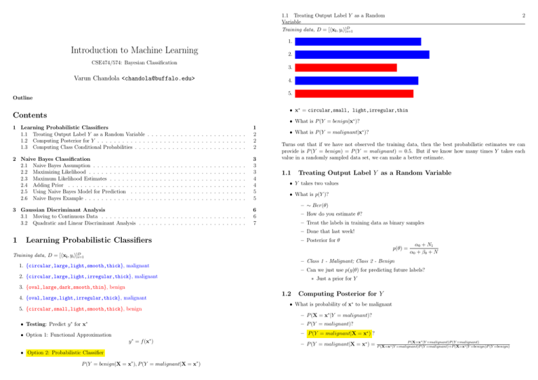
1. {circular,large,light,smooth,thick}, malignant
Introduction to Machine Learning
2. {circular,large,light,irregular,thick}, malignant
CSE474/574: Bayesian Classification
3. {oval,large,dark,smooth,thin}, benign
Varun Chandola <chandola@buffalo.edu>
4. {oval,large,light,irregular,thick}, malignant
5. {circular,small,light,smooth,thick}, benign
Outline
• x∗ = circular,small, light,irregular,thin
Contents
• What is P (Y = benign|x∗ )?
1 Learning Probabilistic Classifiers
1.1 Treating Output Label Y as a Random Variable . . . . . . . . . . . . . . . . . . . . . . . .
1.2 Computing Posterior for Y . . . . . . . . . . . . . . . . . . . . . . . . . . . . . . . . . . . .
1.3 Computing Class Conditional Probabilities . . . . . . . . . . . . . . . . . . . . . . . . . . .
1
2
2
2
2 Naive Bayes Classification
2.1 Naive Bayes Assumption . . . . . . . . .
2.2 Maximizing Likelihood . . . . . . . . . .
2.3 Maximum Likelihood Estimates . . . . .
2.4 Adding Prior . . . . . . . . . . . . . . .
2.5 Using Naive Bayes Model for Prediction
2.6 Naive Bayes Example . . . . . . . . . . .
.
.
.
.
.
.
3
3
3
4
4
5
5
3 Gaussian Discriminant Analysis
3.1 Moving to Continuous Data . . . . . . . . . . . . . . . . . . . . . . . . . . . . . . . . . . .
3.2 Quadratic and Linear Discriminant Analysis . . . . . . . . . . . . . . . . . . . . . . . . . .
6
6
7
.
.
.
.
.
.
.
.
.
.
.
.
.
.
.
.
.
.
.
.
.
.
.
.
.
.
.
.
.
.
.
.
.
.
.
.
.
.
.
.
.
.
.
.
.
.
.
.
.
.
.
.
.
.
.
.
.
.
.
.
.
.
.
.
.
.
.
.
.
.
.
.
.
.
.
.
.
.
.
.
.
.
.
.
.
.
.
.
.
.
.
.
.
.
.
.
.
.
.
.
.
.
.
.
.
.
.
.
.
.
.
.
.
.
.
.
.
.
.
.
.
.
.
.
.
.
.
.
.
.
.
.
.
.
.
.
.
.
.
.
.
.
.
.
.
.
.
.
.
.
.
.
.
.
.
.
.
.
.
.
.
.
• What is P (Y = malignant|x∗ )?
Turns out that if we have not observed the training data, then the best probabilistic estimates we can
provide is P (Y = benign) = P (Y = malignant) = 0.5. But if we know how many times Y takes each
value in a randomly sampled data set, we can make a better estimate.
1.1
Treating Output Label Y as a Random Variable
• Y takes two values
• What is p(Y )?
– ∼ Ber(θ)
– How do you estimate θ?
– Treat the labels in training data as binary samples
– Done that last week!
1
Learning Probabilistic Classifiers
– Posterior for θ
p(θ) =
Training data, D =
[hxi , yi i]D
i=1
– Class 1 - Malignant; Class 2 - Benign
1. {circular,large,light,smooth,thick}, malignant
– Can we just use p(y|θ) for predicting future labels?
2. {circular,large,light,irregular,thick}, malignant
3. {oval,large,dark,smooth,thin}, benign
• Testing: Predict y for x
– P (X = x∗ |Y = malignant)?
∗
• Option 1: Functional Approximation
Computing Posterior for Y
• What is probability of x∗ to be malignant
5. {circular,small,light,smooth,thick}, benign
∗
∗ Just a prior for Y
1.2
4. {oval,large,light,irregular,thick}, malignant
α0 + N1
α 0 + β0 + N
– P (Y = malignant)?
– P (Y = malignant|X = x∗ ) ?
∗
∗
y = f (x )
• Option 2: Probabilistic Classifier
P (Y = benign|X = x∗ ), P (Y = malignant|X = x∗ )
– P (Y = malignant|X = x∗ ) =
P (X=x∗ |Y =malignant)P (Y =malignant)
P (X=x∗ |Y =malignant)P (Y =malignant)+P (X=x∗ |Y =benign)P (Y =benign)
1.3 Computing Class Conditional Probabilities
1.3
3
2.2 Maximizing Likelihood
Computing Class Conditional Probabilities
4
– Joint probability distribution of (X, Y )
• Class conditional probability of random variable X
p(xi , yi ) = p(yi |θ)p(xi |yi )
Y
= p(yi |θ)
p(xij |θjyi )
• Step 1: Assume a probability distribution for X (p(X))
j
• Step 2: Learn parameters from training data
2.2
• But X is multivariate discrete random variable!
Maximizing Likelihood
• Likelihood for D
• How many parameters are needed?
l(D|Θ) =
• 2(2 − 1)
D
i
• How much training data is needed?
j
!
p(xij |θjyi )
ll(D|Θ) = N1 log θ + N2 log(1 − θ)
X
+
N1j log θ1j + (N1 − N1j ) log (1 − θ1j )
j
+
X
j
Naive Bayes Classification
2.1
p(yi |θ)
Y
• Log-likelihood for D
Note that the X can take 2D values. That means that the probability distribution should consist of
probability of observing each possibility. Given that all probabilities sum to 1, we need 2D −1 probabilities.
We need these probabilities for each value of Y , hence 2(2D − 1) probabilities.
Obviously, to reliably estimate the probabilities, one need to observe each possible realization of X at
least a few times. Which means that we need large amounts of training data!
2
Y
N2j log θ2j + (N2 − N2j ) log (1 − θ2j )
• N1 - # malignant training examples, N2 = # benign training examples
• N1j - # malignant training examples with xj = 1, N2j = # benign training examples with xj = 2
Naive Bayes Assumption
• All features are independent
• Each variable can be assumed to be a Bernoulli random variable
P (X = x∗ |Y = malignant) =
∗
P (X = x |Y = benign) =
D
Y
p(x∗j |Y = malignant)
D
Y
p(x∗j |Y
j=1
j=1
P
Derivation of the log-likelihood can be done by using the following results. The summation i log p(yi |θ)
can be expanded and reordered by each class. For each class, the contribution to the sum will be Nc p(yi |θc )
where Nc is the number of P
training
class
Plabel and θc is the class prior for class
P examples with c as the P
c. The double summation i j log p(xij |θjyi ) is same as j i log p(xij |θjyi ). The
P inner sum can be
expanded and order by each class. For each class, the contribution to the sum will be i:yi =c log p(xij |θjc ).
2.3
Maximum Likelihood Estimates
• Maximize with respect to θ, assuming Y to be Bernoulli
= benign)
θ̂ =
y
Nc
N
• Assuming each feature is binary (xj |(y = c) ∼ Bernoulli(θcj ), c = {1, 2})
x1
x2
x3
x4
x5
x6
xD
θ̂cj =
• Only need 2D parameters
• Training a Naive Bayes Classifier
• Find parameters that maximize likelihood of training data
– What is a training example?
∗ xi ?
∗ hxi , yi i
– What are the parameters?
∗ θ for Y (class prior)
∗ θbenign and θmalignant (or θ1 and θ2 )
Algorithm 1 Naive Bayes Training for Binary Features
1:
2:
3:
4:
5:
6:
7:
8:
9:
10:
11:
12:
Nc = 0, Ncj = 0, ∀j
for i = 1 : N do
c ← yi
Nc ← Nc + 1
for j = 1 : D do
if xij = 1 then
Ncj ← Ncj + 1
end if
end for
end for
N
θ̂c = NNc , θ̂cj = Ncjc
return b
Ncj
Nc
2.4 Adding Prior
2.4
5
3. Gaussian Discriminant Analysis
• Test example: x∗ = {cir, small, light}
Adding Prior
• Add prior to θ and each θcj .
We can predict a label in three ways. First is to use the MLE for all the parameters. Second is to use
MAP and third is to use the Bayesian averaging approach. In each, we need to plug in the parameter
estimates in:
– Beta prior for θ (∼ Beta(a0 , b0 ))
– Beta prior for θcj (∼ Beta(a, b))
P (Y = malignant|X = x∗ ) = θ̂ × θ̂malignant,cir × θ̂malignant,small × θ̂malignant,light
P (Y = benign|X = x∗ ) = θ̂ × θ̂benign,cir × θ̂benign,small × θ̂benign,light
Posterior Estimates
p(θ|D) = Beta(N1 + a0 , N − N1 + b0 )
p(θcj |D) = Beta(Ncj + a, Nc − Ncj + b)
2.5
6
Using Naive Bayes Model for Prediction
p(y = c|x∗ , D) ∝ p(y = c|D)
• MLE approach, MAP approach?
Y
j
p(x∗j |y = c, D)
• Bayesian approach:
p(y = 1|x, D) ∝
Z
Ber(y = 1|θ)p(θ|D)dθ)
Y Z
Ber(xj |θcj )p(θcj |D)dθcj
j
N1 + a0
θ̄ =
N + a0 + b 0
3
Gaussian Discriminant Analysis
3.1
Moving to Continuous Data
• Naive Bayes is still applicable!
• Each variable is a univariate Gaussian (normal) distribution
p(y|x) = p(y)
Y
j
= p(y)
p(xj |y) = p(y)
1
(2π)D/2 |Σ|1/2
Y
j
−
1
q
e
2
2πσj
(xj −µi )2
2σ 2
j
(x−µ)> Σ−1 (x−µ)
−
2
e
2
• Where Σ is a diagonal matrix with σ12 , σ12 , . . . , σD
as the diagonal entries
• µ is a vector of means
• Treating x as a multivariate Gaussian with zero covariance
• Gaussian Discriminant Analysis
– Class conditional density
p(x|y = 1) = N (µ1 , Σ1 )
p(x|y = 2) = N (µ2 , Σ2 )
– Posterior density for y
θ̄cj =
Ncj + a
Nc + a + b
Obviously, the MLE and MAP approach use the MLE and MAP estimates of the parameters to compute
the above probability.
2.6
#
1
2
3
4
5
6
7
8
9
10
Naive Bayes Example
Shape
cir
cir
cir
ovl
ovl
ovl
ovl
ovl
cir
cir
Size
large
large
large
large
large
small
small
small
small
large
Color
light
light
light
light
dark
dark
dark
light
dark
dark
Type
malignant
benign
malignant
benign
malignant
benign
malignant
benign
benign
malignant
p(y = 1|x) =
p(y = 1)N (µ1 , Σ1 )
p(y = 1)N (µ1 , Σ1 ) + p(y = 2)N (µ2 , Σ2 )
• Mahalanobis distance of x from the two means.
One can geometrically interpret the Gaussian Discriminant Analysis by noting that the exponential in the
pdf of a multivariate gaussian:
(x − µ)> Σ−1 (x − µ)
is the Mahalanobis Distance between an example x and the mean µ in the D dimensional space. For
better understanding let us consider the Eigendecomposition of Σ, i.e., Sigma = UΛU> , where U is an
orthonormal matrix of eigenvectors with U> U = I and Λ is a diagonal matrix consisting of eigenvalues.
We can rewrite the inverse of Σ as:
Σ−1 = (UΛU> )−1
= U−1 Λ−1 U−>
D
X
1
=
ui u>
i
λ
i=1 i
3.2 Quadratic and Linear Discriminant
7
Analysis
where ui is the ith eigenvector and λi is the corresponding eigenvalue. The Mahalanobis distance between
x and µ can be rewritten as:
!
D
X
1
> −1
>
>
(x − µ) Σ (x − µ) = (x − µ)
ui ui (x − µ)
λ
i=1 i
=
=
D
X
1
(x − µ)> ui u−1
i (x − µ)
λ
i=1 i
D
X
y2
i
i=1
λi
>
where yi = (x − µ) ui . This is an equation for an ellipse in D-dimensional space. Thus it shows that the
points on an ellipse around the mean have the same probability density for a Gaussian.
3.2
Quadratic and Linear Discriminant Analysis
• Using non-diagonal covariance matrices for each class - Quadratic Discriminant Analysis (QDA)
– Quadratic decision boundary
• If Σ1 = Σ2 = Σ
• Linear Discriminant Analysis (LDA)
– Parameter sharing or tying
– Results in linear surface
– No quadratic term
References