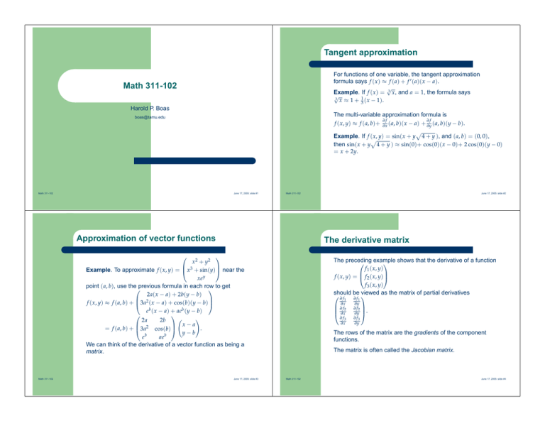
Tangent approximation
For functions of one variable, the tangent approximation
formula says f (x) ≈ f (a) + f 0 (a)(x − a).
√
Example. If f (x) = 3 x, and a = 1, the formula says
√
3
x ≈ 1 + 13 (x − 1).
Math 311-102
Harold P. Boas
The multi-variable approximation formula is
∂f
∂f
f (x, y) ≈ f (a, b)+ ∂x (a, b)(x − a) + ∂y (a, b)(y − b).
p
Example. If f (x, y) = sin(x + y 4 + y ), and (a, b) = (0, 0),
p
then sin(x + y 4 + y ) ≈ sin(0)+ cos(0)(x − 0)+ 2 cos(0)(y − 0)
= x + 2y.
boas@tamu.edu
Math 311-102
June 17, 2005: slide #1
Math 311-102
Approximation of vector functions
The derivative matrix

x 2 + y2


Example. To approximate f (x, y) =  x3 + sin(y)  near the
xey
point (a, b), use theprevious formula in each row
 to get
2a(x − a) + 2b(y − b)


f (x, y) ≈ f (a, b) + 3a2 (x − a) + cos(b)(y − b) 
b
b
e (x − a) + ae (y − b)


Ã
!
2a
2b
 x−a
 2
.
= f (a, b) + 3a cos(b)
y−b
eb
aeb
We can think of the derivative of a vector function as being a
matrix.

Math 311-102
June 17, 2005: slide #2
June 17, 2005: slide #3
The preceding
example
 shows that the derivative of a function

f 1 (x, y)


f (x, y) =  f 2 (x, y)
f 3 (x, y)
should
be
viewed
as the matrix of partial derivatives


∂ f1
 ∂∂xf2

 ∂x
∂ f3
∂x
∂ f1
∂y
∂ f2 

∂y .
∂ f3
∂y
The rows of the matrix are the gradients of the component
functions.
The matrix is often called the Jacobian matrix.
Math 311-102
June 17, 2005: slide #4
Exercise
Answers

4
sin(x) + 12
25 tan(y) + 5 z

16
3 z 
f (x, y, z) =  12

25 x + 25 sin(y) − 5 ze
4
3
− 5 x cos(x) + 5 y + yz

9
25
1.
 The Jacobian matrix equals
9
12
2
25 cos(x)
25 sec (y)

12
16

25
25 cos(y)
3
− 45 cos(x) + 45 x sin(x)
5 +z


1. Find the derivative matrix of f at (0, 0, 0).
2. Show that the matrix is orthogonal: the inverse equals the
transpose.

=
3. The matrix is a rotation matrix. Find the axis of rotation.
9
25
12
25
− 45
12
25
16
25
3
5
4
5
3 .
−5
4
5
¯
¯
¯
3 z
3 z ¯
− 5 e − 5 ze ¯
¯
¯
y
(0,0,0)
0
2. The columns of the matrix are orthonormal.
 
3
 
3. The vector 4 is an eigenvector with eigenvalue 1.
0
Math 311-102
June 17, 2005: slide #5
Math 311-102
June 17, 2005: slide #6