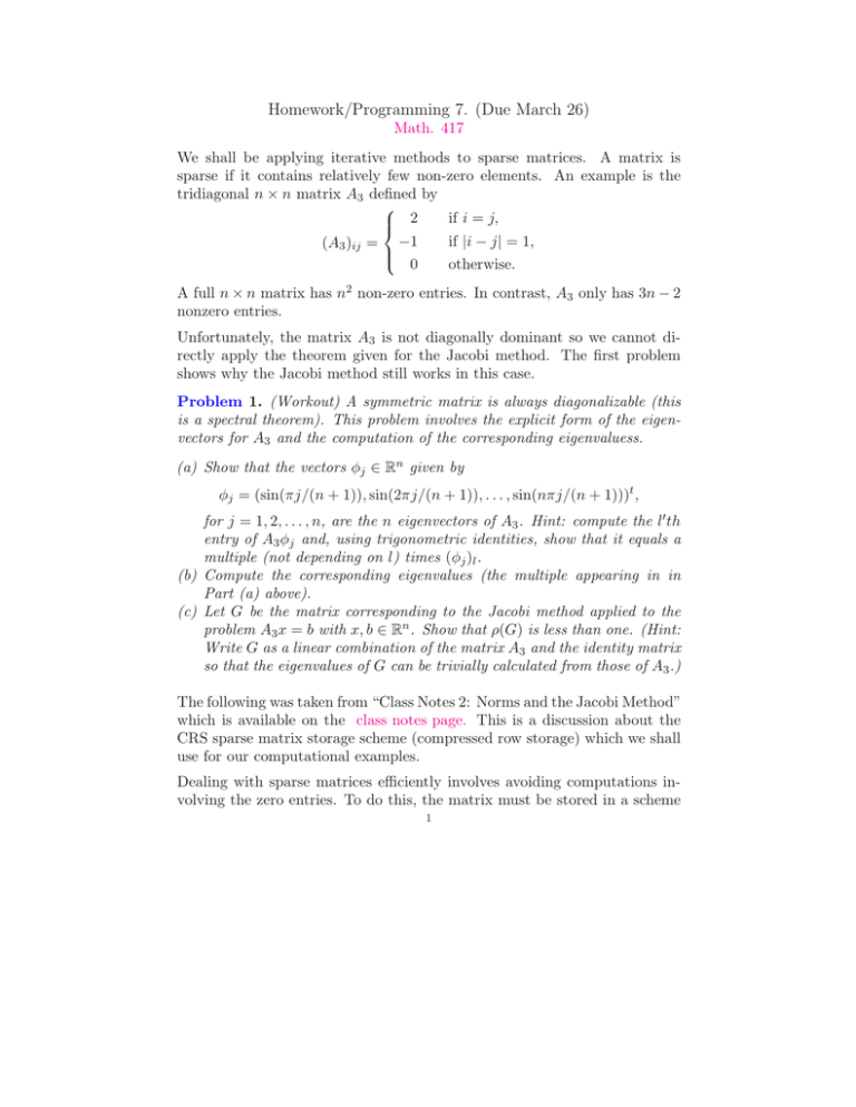
Homework/Programming 7. (Due March 26)
Math. 417
We shall be applying iterative methods to sparse matrices. A matrix is
sparse if it contains relatively few non-zero elements. An example is the
tridiagonal n × n matrix A3 defined by

if i = j,

 2
if |i − j| = 1,
(A3 )ij = −1

 0
otherwise.
A full n × n matrix has n2 non-zero entries. In contrast, A3 only has 3n − 2
nonzero entries.
Unfortunately, the matrix A3 is not diagonally dominant so we cannot directly apply the theorem given for the Jacobi method. The first problem
shows why the Jacobi method still works in this case.
Problem 1. (Workout) A symmetric matrix is always diagonalizable (this
is a spectral theorem). This problem involves the explicit form of the eigenvectors for A3 and the computation of the corresponding eigenvaluess.
(a) Show that the vectors φj ∈ Rn given by
φj = (sin(πj/(n + 1)), sin(2πj/(n + 1)), . . . , sin(nπj/(n + 1)))t ,
for j = 1, 2, . . . , n, are the n eigenvectors of A3 . Hint: compute the l′ th
entry of A3 φj and, using trigonometric identities, show that it equals a
multiple (not depending on l) times (φj )l .
(b) Compute the corresponding eigenvalues (the multiple appearing in in
Part (a) above).
(c) Let G be the matrix corresponding to the Jacobi method applied to the
problem A3 x = b with x, b ∈ Rn . Show that ρ(G) is less than one. (Hint:
Write G as a linear combination of the matrix A3 and the identity matrix
so that the eigenvalues of G can be trivially calculated from those of A3 .)
The following was taken from “Class Notes 2: Norms and the Jacobi Method”
which is available on the class notes page. This is a discussion about the
CRS sparse matrix storage scheme (compressed row storage) which we shall
use for our computational examples.
Dealing with sparse matrices efficiently involves avoiding computations involving the zero entries. To do this, the matrix must be stored in a scheme
1
2
which only involves the nonzero entries. We shall use a modified “Compressed Sparse Row” (CSR) structure. A nice discussion of compressed
sparse row structure can be found at
http://www.cs.utk.edu/∼dongarra/etemplates/node373.html.
This structure is designed so that it is easy to access the entries in a row.
Our modification is made so that it is also easy to access the diagonal entry
in any row.
The CSR structure involves three arrays, VAL, CIND and RIND. VAL is an
array of real numbers and stores the actual (nonzero) entries of A. CIND is
an integer array which contains the column indexes for nonzero entries in A.
The length of VAL and CIND are equal to the number of nonzero entries in
A. Finally, RIND is an integer array of dimension n+1 and contains the row
offsets (into the arrays VAL and CIND). By convention, RIND(n+1) is set to
the total number of nonzeroes plus one. This structure should become clear
by examining the following example (see also the URL above). Consider


2
−1
0
0
−1/3
3
−2/3
0 
.
A=
 0
−1/4
4
−3/4
0
0
−1/5
5
The modified CSR structure is as follows:
VAL
2
−1 3 −1/3 −2/3 4 −1/4 −3/4 5
−1/5
CIND
1
2 2
1
3
3
2
4
4
3
and
RIND 1 3 6 9 11.
Note that the i’th entry of RIND points to the start of the nonzero values
(in VAL) for the i’th row. It also points to the start of the column indexes
for that row. The modification is that we always put the diagonal entry
at that location, i.e. VAL(RIND(i))=Ai,i . The general CSR structure does
not do this. In fact, the general CSR storage scheme does not even have a
diagonal entry whenever the diagonal entry is zero. However, we will always
be considering matrices with nonzero diagonal entries (so that we can apply
the Jacobi, Gauss-Seidel and SOR iterative methods).
Problem 2. (Workout) Write down the arrays VAL, CIND and RIND corresponding to the matrix A3 when n = 6.
3
From this point on, we shall only be applying iterative methods to sparse
matrices in CRS form which will be provided through input files. A MATLAB m-file function for reading a CRS matrix data file is given in readcrs.m.
Its interface is given by:
function [n,nnzero,rind,cind,val]=readcrs(filename).
Given the file name, the function returns values a CRS stored n×n matrix A
with nnzero non-zero entries defining the arrays rind, cind, val as discussed
above.
Problem 3. (MATLAB) Write a matlab m-file function which does one
step of the Jacobi method. This function has the arguments:
(a) n, rind, cind, val representing the CRS matrix,
(b) a vector xi (the i’th iterate),
(c) A vector b (the right had side of Ax = b),
and returns xip where
(3.1)
xip = xi + D−1 (b − A ∗ xi).
To implement the above line, use the equivalent CRS form illustrated below:
function [xip]=jacobi(n,rind,cind,val,xi,b)
for i=1:n
s=b(i)
for j in (1...n) such that A_ij not equal 0 and j not equal i
s=s-A_ij * xi(cind(j));
end
xip(i)=s/A_ii;
end
Further Discussion: Note that xi(j) was incorrect in an earlier version of this assignment and has been corrected above (xi(cind(j))).
This typo should have been obvious if you attended recitation (and
also from the A-evaluation routine on Jun Ren’s homepage).
4
Upon first examination, it may appear that the above code does
not implement the iteration (3.1). To see that it does, we rewrite
(3.1) as:
X
X
xip(i) = xi(i)+A−1
Aij xi(j)−Aii xi(i)) = A−1
Aij xi(j)).
ii (b(i)−
ii (b(i)−
j6=i
j6=i
Of course, you need to convert the above to code acceptable to MATLAB and
use the CRS structure to determine which indexes are included in the second
for loop as well as the values of Aij .
Since the Jacobi method is linear, the convergence is determined by the error
behavior which is given by the formula ei+1 = Gei . Thus, to numerically
study the error behavior of the method, we can solve a problem with right
hand side 0 and initial iterate x0 6= 0. In this case, ei = −xi and so ei and
xi have the same norm.
Problem 4. (MATLAB) Write a driver routine for doing the Jacobi iteration on the problem Ax = 0 with A given in CRS form (do not assemble the full matrix A under any circumstances) and initial iterate x0 = (1, 1, 1, . . . , 1)n . After each step in your iteration, compute
√
kei k2 := ei · ei and continue iteration until the relative error is less than ǫ,
i.e.
kei k2 /ke0 k2 < ǫ.
Using the above driver, run the Jacobi method applied to the matrices coming
from the CRS sparse matrix files below.
(a) a3-8.txt
(b) a3-16.txt
(c) a3-32.txt
(d) a3-64.txt
(e) a3-128.txt
(f ) a3-256.txt
to approximate the solution to Ax = 0 with initial iterate given by x0 =
(1, 1, 1, . . . , 1)t . The driver code should look like
5
.
[n,nzero,rind,cind,val]=readcrs("filename");
.
i=0; % iteration counter
repeat
xip=jacobi(n,rind,cind,val,xi,b);
i=i+1;
relnorm=...
xi=xip;
until relnorm<epsilon
end
print(i,relnorm);
% the number of iterations required.
Further discusssion: To make things clearer, I have slightly modified the driver code above.
For each of the six files report
n
in
relnormin
(1 − ρ(Gn ))−1 .
Here in is the iteration when relnormin becomes less than ǫ := .0001 where
relnormi := kei k2 /ke0 k2 .
Also, ρ(Gn ) is the spectral radius of the n × n matrix A3 (computed in Problem 1).
Further Discussion: Some students may be having trouble dealing
with the files. You need to get all files into a common subdirectory
(e.g., the data files, the readcrs.m file and your homework m-file)
and run matlab in that subdirectory. The easiest solution is to use
your home directory on calclab machines. Matlab runs in your
main subdirectory when you click on it. Now using Netscape on
calclab, when you click on the file readcrs.m (while visiting the
homework 7 page), Netscape will save the file in the Downloads
folder. The easiest way to move it into your main directory is to
open a terminal (looks like a computer display) and type
mv Downloads/readcrs.m .
Note that the ending period above is part of the command. To
get a txt file, you again click on it while visiting the h7 page using
6
Netscape.
right click
allows you
saved (use
Netscape brings up a copy of the file and you need to
in the body and select “Save file as.” Netscape then
to navigate to the subdirectory where the file is to be
your home directory but do not change the file name).
I cannot give instructions for other computer systems or browsers
as, although they all have the capability, the syntax is not uniform.
Hand in the results for Problems 1,2 and 4 and a copy of the
matlab code for Problems 3 and 4.