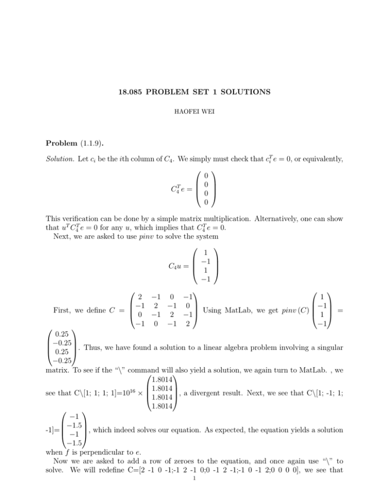
18.085 PROBLEM SET 1 SOLUTIONS
HAOFEI WEI
Problem (1.1.9).
Solution. Let ci be the ith column of C4 . We simply must check that cTi e = 0, or equivalently,
 
0

0 

C4T e = 
 0 
0
This verification can be done by a simple matrix multiplication. Alternatively, one can show
that uT C4T e = 0 for any u, which implies that C4T e = 0.
Next, we are asked to use pinv to solve the system


1
 −1 

C4 u = 
 1 
−1

 
1
2 −1 0 −1
−1
−1 2 −1 0 

 
First, we define C = 
 0 −1 2 −1 Using MatLab, we get pinv (C)  1  =
−1
−1 0 −1 2


0.25
−0.25


 0.25 . Thus, we have found a solution to a linear algebra problem involving a singular
−0.25
matrix. To see if the “\” command
 willalso yield a solution, we again turn to MatLab. , we
1.8014

1.8014

see that C\[1; 1; 1; 1]=1016 × 
1.8014, a divergent result. Next, we see that C\[1; -1; 1;
1.8014


−1
−1.5

-1]=
 −1 , which indeed solves our equation. As expected, the equation yields a solution
−1.5
when f is perpendicular to e.
Now we are asked to add a row of zeroes to the equation, and once again use “\” to
solve. We will redefine C=[2 -1 0 -1;-1 2 -1 0;0 -1 2 -1;-1 0 -1 2;0 0 0 0], we see that

1
HAOFEI WEI
18.085 PROBLEM SET 1 SOLUTIONS

−0.0802
−0.2355

C\[1;1;1;1;0]=10− 15 × 
−0.5023 ≈ 0, which also fails as a solution. However, C\[1;-1;1;0
 
0.5
0

1;0]=
0.5, which is also a possible solution.
0

Problem (1.1.16).
Solution. The first method of multiplication is by rows, which gives
2 3
4 5
1
1×2+2×3
8
=
=
2
1×4+2×5
14
The second method uses multiplication by columns, which gives
2 3
1
2
3
8
=1×
+2×
=
4 5
2
4
5
14
Problem (1.1.27). Note: this problem can be found in the online version of chapter 1 of the
book




−1 1
0 0
2 −1 0
Solution. Given A0 =  0 −1 1 0, we are asked to show A0 AT0 = K3 = −1 2 −1.
0
0 −1 1
0 −1 2
It is an elementary multiplication which may be done in MatLab, and from that multiplication we see that A0 AT0 = K3 .


1
0 0
In order to get T3 , we would delete the first column of A0 to get A1 = −1 1 0.
0 −1 1


1 −1 0
Using MatLab again, we can see that A1 AT1 = T3 = −1 2 −1.
0 −1 2


1
0
Finally, we can delete the last column of A1 to get A2 = −1 1 . Finally, using
0 −1


1 −1 0
MatLab, we will get A2 AT2 = B3 = −1 2 −1.
0 −1 1
Problem (1.2.4).
2
HAOFEI WEI
18.085 PROBLEM SET 1 SOLUTIONS
1
0
−1 1
Solution. We have two matrices, ∆− = 
..

.



1
1

= . . .



1

0


and
M
.
sum
..
1 1

. 0
.
.. 1 1
−1 1
1
To check that the two matrices are inverses, we must verify that ∆− Msum = Msum ∆− = I.
The first order of multiplication gives
i−1,j
i,j
Let A = ∆− Msum . We see element aij,i>1 of A can be given by −Msum
+ Msum
. For
i > j, both summands are 0, whereas for i < j, both summands are equal to 1, resulting in
a sum of 0 in both cases. For i = j, the first summand is 0 and the second summand is 1,
resulting in a sum of 1. Finally, for i = 1, we see with simple multiplication that a11 = 1
and ai,j>1 = 0. Thus, A = I.
nj
Now let B = Msum ∆− . Element bij of B can be given by Σn=i
n=1 ∆− . For i < j, the total
sum comes out to be −1 + 1 = 0, whereas for i > j, all the summands are 0. For i = j, the
only nonzero summand will be 1, giving us B = I. From these two multiplications, we see
that ∆− and Msum are inverses.
Next, we are asked to find ∆0 = 12 (∆+ + ∆− ). Through simple matrix addition, we find
that



−1 1
0
1
 1 −1 0
  0 −1 1

1
0
= 
+

.. ..
..
.




2
. 1
.
. 0
−1 . . 1
0 −1
−1 1
−1 0
 

u1
0
1 0
For n = 3, we have ∆0 u = 12 −1 0 1 u2  = 0. By inspection, we can see that
u3
0 −1 0
 
1
u1 = u3 and u2 = 0. Thus, any solution of the form a × 0, where a is any number, will
1
solve the system.

 
0
1
0
0 0
u1
−1 0
 u 2 
1
0
0

 
 u3  = 0. Again by inspection,
0
−1
0
1
0
For n = 5, we have ∆0 u = 21 

 
0
0 −1 0 1 u4 
0
0
0 −1 0
u5
 
1
0
 

we can see that u2 = u4 = 0 and u1 = u3 = u5 . Thus, any solution of the form a × 
1, a
0
1
any number, will solve the system.
1
0
−1 1

..

.



Problem (1.2.7).
3
HAOFEI WEI
18.085 PROBLEM SET 1 SOLUTIONS
Solution. First, we will consider the u = 1 case. In this case, u0 = 0, and the approximation
gives
−1 + 8 − 8 + 1
=0
12h
Next, we will consider the u = x2 case. In this case, u0 = 2x, and the approximation gives
−(x + 2h)2 + 8(x + h)2 − 8(x − h)2 + (x − 2h)2
12h
1
=
× −x2 − 4xh − 4h2 + 8x2 + 16h + 8h2 − 8x2 + 16xh − 8h2 + x2 − 4h + 4h2
12h
(32 − 8)xh
= 2x
=
12h
which matches our exact solution.
Finally, we will consider the u = x4 case. In this case, u0 = 4x3 , and the approximation
gives
=
=
=
=
−(x + 2h)4 + 8(x + h)4 − 8(x − h)4 + (x − 2h)4
12h
1
[(x − 2h)2 + (x + 2h)2 ][(x − 2h)2 − (x + 2h)2 ] + 8[(x + h)2 + (x − h)2 ][(x + h)2 − (x − h)2
12h
1 2
(2x + 8h2 )(−8xh) + 8(2x2 + 2h2 )(4xh)
12h
(−16 − 64 + 64 + 64)xh2
12h
4x3
which again matches our exact solution.
Note that in the above cases, the error is 0 because the 5th derivative of all these functions
are 0.
We must also find the coefficient b of the 5th order error. To do this, we must use
Taylor series expansions of u. To that end, we only need to consider the 5th order terms in
5 d5 u
the Taylor expansions of u(x + 2h), u(x + h), u(x − h), and u(x − 2h), which are 32h
,
120 x5
h5 d5 u
h5 d5 u
32h5 d5 u
, − 120 x5 , and − 120 x5 respectively for the 4 functions. Plugging these into our
120 x5
4
h5
−48h5
approximation equation, we get bh4 = 12h×120
(−32 + 8 + 8 − 32) = 12h×120
= − h30 . Thus,
b = −1
.
30
Problem (1.2.18).
Solution. For a second order finite difference approximation with boundary conditions u(0) =
u(1) = 0, K is the proper matrix to use to approximate the second derivative. Since we
have n = 4, we must have 4 points between 0 and 1, meaning
  we will have a stepsize of
1

2

h = 1/5. Thus, the equation we must solve is − h12 Ku = h 
3. Note here −K is used as
4
d2 u
K is actually the matrix for − dx2 . Since K is not a singular matrix, we can use MatLab’s
4
HAOFEI WEI
18.085 PROBLEM SET 1 SOLUTIONS
“\” to easily solve this matrix equation. Using MatLab, we will find that

  
2 −1 0
0
1




−1
2
−1
0
 \ 2
u = −h3 
 0 −1 2 −1 3
0
0 −1 2
4
 
4

1 
7
= −

125 8
6
To find the exact solution, we will simply integrate the differential. After integrating, we
have u = − 16 x3 + Cx + D. To fit the initial condition u(0) = 0, we see D = 0. To fit the
initial condition u(1) = 0, we see that C = − 16 . Thus,
the exact solution of
this
 equation
 
1
4
2
 
, we get u = − 1 7, exactly
is u(x) = − 61 x3 − 16 x. Plugging in values of x = 15 
125 8
3
4
6
matching our finite difference method.
The reason that we have an exact match between the two solutions is because the finite
difference method, as we saw in an earlier problem, has an error proportional to the 5th
derivative of the function. For our function, the 5th derivative is 0, so there is no error
between the exact and finite difference methods.
5