IJMMS 29:3 (2002) 143–153
PII. S0161171202011055
http://ijmms.hindawi.com
© Hindawi Publishing Corp.
FIXED-WIDTH CONFIDENCE INTERVAL FOR A LOGNORMAL MEAN
MAKOTO AOSHIMA and ZAKKULA GOVINDARAJULU
Received 25 October 2000
We consider the problem of constructing a fixed-width confidence interval for a lognormal
mean. We give a Birnbaum-Healy type two-stage procedure to construct such a confidence
interval. We discuss some asymptotic properties of the procedure. A three-stage procedure
and an accelerated sequential procedure are also given for the comparison of efficiency
among these three multistage methodologies.
2000 Mathematics Subject Classification: 62L12, 62L10.
1. Introduction. Suppose there is a lognormal distribution with unknown parameters µ and σ 2 . Let X1 , X2 , . . . be a random sequence from this distribution. Then
Y1 , Y2 , . . . is a random sequence from N(µ, σ 2 ), where Yi = ln Xi , i = 1, 2, . . . . The
mean of the lognormal distribution is a nonlinear function of (µ, σ 2 ) as E(X) =
exp(µ + σ 2 /2) (= θ, say) and it is unknown since µ and σ 2 are unknown. Also,
note that V (X) = {exp(σ 2 ) − 1} exp(2µ + σ 2 ). Let θn be an estimator of θ based on
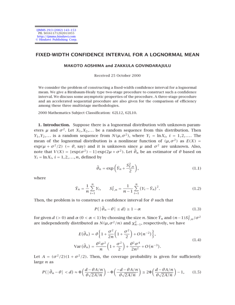
Yi = ln Xi , i = 1, 2, . . . , n, defined by
SY2 ,n
θn = exp Ȳn +
,
2
(1.1)
where
Ȳn =
n
1 Yi ,
n i=1
SY2 ,n =
n
2
1 Yi − Ȳn .
n − 1 i=1
(1.2)
Then, the problem is to construct a confidence interval for θ such that
P θn − θ ≤ d ≥ 1 − α
(1.3)
for given d (> 0) and α (0 < α < 1) by choosing the size n. Since Ȳn and (n−1)SY2 ,n /σ 2
2
are independently distributed as N(µ, σ 2 /n) and χn−1
, respectively, we have
σ2
σ2
E θn = θ 1 +
1+
+ O n−2 ,
2n
2
2
2
2
θ σ
σ
θ2 σ 4
+ O n−3 .
1+
+
Var θn =
n
2
2n2
(1.4)
Let A = (σ 2 /2)(1 + σ 2 /2). Then, the coverage probability is given for sufficiently
large n as
d − θA/n
−d − θA/n
d − θA/n
P θn − θ < d ≈ Φ
−Φ
≥ 2Φ
− 1,
(1.5)
θ 2A/n
θ 2A/n
θ 2A/n
144
M. AOSHIMA AND Z. GOVINDARAJULU
where Φ(·) denotes the N(0, 1) distribution function. Hence, it is easy to see that the
requirement (1.3) is satisfied asymptotically when d is small if n is chosen as
n≥
2θA d + θz2
2
d
= n , say ,
(1.6)
where z is the upper point α/2 of the N(0, 1) distribution, that is, Φ(z) = 1−α/2. That
is, n given by (1.6) is an asymptotically optimal sample size and the requirement
(1.3) is satisfied only if θ 2 A2 /n2 → 0 for large n. However, the fixed-sample size n is
unknown since µ and σ 2 are unknown.
Takada [16] showed that there is no fixed-sample size procedure to construct a
fixed-width confidence interval for the mean of lognormal distribution with at least
the nominal value uniformly for all µ and σ 2 . So, we resort to some sequential methodology for this problem. Takada gave a solution to this problem by extending Nagao’s
[13] sequential procedure to a Birnbaum-Healy-type two-stage procedure. However,
the procedure given there tends to require very large sample sizes in order to meet
the requirement (1.3). In this paper, we give a two-stage procedure which is also a
Birnbaum-Healy-type two-stage procedure, but it is more efficient than Takada’s procedure. For the reference on other applications of Birnbaum-Healy-type two-stage procedure, see Graybill and Connell [8, 9] and Govindarajulu [5, 6, 7]. For the original idea
of sequential sampling in two stages, see Stein [15] and Cox [4].
In Section 2, a two-stage procedure is given for constructing a confidence interval
which satisfies (1.3) asymptotically. In Section 3, some asymptotic properties of the
procedure are discussed when compared with Takada’s procedure asymptotically. In
Sections 4 and 5, we give a three-stage procedure and an accelerated sequential procedure for this problem. Finally, in Section 6, a Monte-Carlo study is presented to
compare the efficiency among these three multistage procedures for moderate samples.
2. Two-stage procedure. We first take the preliminary sample X1 , . . . , Xm of size
m (≥ 2) and compute
b
θm = exp a + Ȳm + SY2 ,m ,
2
m =
A
bSY2 ,m
2
1+
bSY2 ,m
2
,
(2.1)
where Ȳm and SY2 ,m are defined like (1.2), and the constants a (≤ 0) and b (≥ 1) are
determined later so as to satisfy the requirement (1.3) asymptotically. Next, we take
the second sample Xm+1 , . . . , Xm+N of size N defined by using (2.1) as
N=
m 2θm A
2
d + θm z
+ 1,
d2
(2.2)
where [x] denotes the largest integer less than x. Then, a confidence interval for θ is
constructed by using θN defined as (1.1) on the basis of the second sample of size N.
The coverage probability (CP) is given for sufficiently large N by
d − θA/N
d − θA/N
−d − θA/N
CP ≈ E Φ
≥ 2E Φ
− 1.
−Φ
θ 2A/N
θ 2A/N
θ 2A/N
(2.3)
FIXED-WIDTH CONFIDENCE INTERVAL FOR A LOGNORMAL MEAN
We determine the design constants a and b so as to satisfy
α
d − θA/N
≥ 1− .
E Φ
2
θ 2A/N
145
(2.4)
In order to meet the requirement (1.3) asymptotically, we write that
E Φ
d − θA/N
θ 2A/N
=E Φ
−
δ
2
1/2
m
θm A
θm 2
δ+
z
θ A
θ
−1/2 m
θm A
θm 2
δ+
z
,
θ A
θ
where δ = d/θ. Since it increases as δ increases, we have

 
m A
m
θ
.
Equation(2.5) ≥ E Φz
θ
A
(2.5)
(2.6)
We note that


θm
σ2
σ2
σ2

= exp
Z +a+
(bW − 1) ≈ exp a +
(bW − 1)
θ
m
2
2
(2.7)
for sufficiently large m, and
m
bW 2 + bW σ 2
A
,
=
A
2+σ2
(2.8)
where Z and νW are independently distributed as the N(0, 1) and χν2 with ν = m − 1,
respectively. Then, we write the right-hand side of (2.6) for sufficiently large m as
∞ bW 2 + bW σ 2
σ2
Φ z exp a +
(2.9)
(bW − 1)
gν (W )dW ,
2
2+σ2
0
where gν (·) denotes the density function of the random variable χν2 /ν. We set h(σ 2 ) =
z exp(a + (σ 2 /2)(bW − 1)) bW (2 + bW σ 2 )/(2 + σ 2 ). Then, since minσ 2 >0 h(σ 2 ) =
√
zea bW for 1/b < W < ∞ and minσ 2 >0 h(σ 2 ) = 0 for 0 < W < 1/b, we obtain that
Integral(2.9) ≥
∞
1
Φ zea bW gν (W )dW +
2
1/b
1/b
0
gν (W )dW .
So, we use the constants a and b such that
∞
1 1/b
α
Φ zea bW gν (W )dW +
gν (W )dW = 1 − .
2 0
2
1/b
(2.10)
(2.11)
√
1/b
∞
Since 1/b Φ(zea bW )gν (W )dW → (1/2)(1 − α/2) and 0 gν (W )dW → 1 − α/2 as
m → ∞, we consider (a, b) satisfying
∞
α
1
1−
,
(2.12)
Φ zea bW gν (W )dW =
2
2
1/b
1/b
α
gν (W )dW = 1 − .
(2.13)
2
0
146
M. AOSHIMA AND Z. GOVINDARAJULU
However, we can see that there is no solution to (2.12) when m < ∞, because
√
∞
a
bW )gν (W )dW increases in m since
1/b Φ(ze
∞
1/b
∞
Φ zea bW gν (W )dW ≈ √
ν/2(1/b−1)
Φ zea b φ(Z)dZ
(2.14)
for sufficiently large m, where φ(·) denotes the N(0, 1) density function. So, we determine the constants a and b as follows: by using the normal approximation to νW
for sufficiently large ν, the left-hand side of (2.11) is written as


∞
! 2
ν 1
1
a

Z + 1 φ(Z)dZ + Φ
−1 .
(2.15)
Φ ze b
√
ν
2
2 b
ν/2(1/b−1)
Now we consider that a and b are sequences depending on m such that a → 0, b → 1
as m → ∞. Let ν = m − 1 (sufficiently large),
k
a= √ ,
ν
b = 1− √ ,
ν
(2.16)
√
where k and (< −3 2) are constants, and expand (2.15) such that
√
∞ 1
2Z − 1
1
φ(Z)dZ √ + Φ √
+o √ .
+ zφ(z) √ k +
Φ(z) 1 − Φ √
2
ν 2
ν
2
2
/ 2
(2.17)
In the second term of the above expansion, we let
√
∞ 2Z − k
+
φ(Z)dZ = 0.
(2.18)
√
2
/ 2
Then, we have
k=
√ √ 1/ 2 φ / 2
√ +
2
Φ / 2 − 1
= f (), say
(2.19)
and from (2.16)
f
f ()
a= √ =
ν
√ ν 1/b − 1
√
.
ν
(2.20)
To calculate the values of a and b, we first substitute the constant a given by (2.20)
into (2.11). Then, we obtain the value of b by solving (2.11) for given (α, m) with the
bisection method. The value of a is given by (2.20) with b determined above. Here,
the 128-point Gauss-Legendre numerical quadrature formula was used to evaluate the
left-hand side of (2.11). Since the integral
∞
Φ zea bW gν (W )dW
= h(a, b), say
(2.21)
1/b
is over an infinite range, we instead calculate
u
1/b
Φ zea bW gν (W )dW
= hu (a, b), say .
(2.22)
FIXED-WIDTH CONFIDENCE INTERVAL FOR A LOGNORMAL MEAN
We choose the constant u such that
ε ≥ h(a, b) − hu (a, b) ≥ 0,
147
(2.23)
for given ε (> 0). Since
h(a, b) − hu (a, b) =
∞
u
Φ zea bW gν (W )dW ≤
∞
u
gν (W )dW = 1 − Gν (uν),
(2.24)
where Gν (·) denotes the χν2 distribution function, we have
u=
Gν−1 (1 − ε)
ν
(2.25)
satisfying (2.23) for given ε (> 0). Table 2.1 gives the values of a and b for given m
(= ν + 1) = 20(20)100(100)500 and α = 0.01, 0.05, and 0.10. This table was obtained
by setting ε = 10−5 .
Table 2.1. The values of a and b for given m and α (the upper entry is for
a and the lower entry is for b).
α\m
0.01
0.05
0.10
20
40
60
80
100
200
300
400
−0.332
−0.259
−0.223
−0.200
−0.184
−0.141
−0.120
−0.107
−0.098
500
2.819
2.043
1.792
1.661
1.578
1.391
1.315
1.272
1.243
−0.302
−0.234
−0.201
−0.181
−0.166
−0.128
−0.109
−0.097
−0.089
2.354
1.836
1.653
1.553
1.489
1.339
1.277
1.240
1.216
−0.288
−0.223
−0.192
−0.173
−0.159
−0.122
−0.104
−0.093
−0.085
2.189
1.758
1.599
1.511
1.454
1.319
1.262
1.228
1.205
Note that a → 0 and b → 1 as m → ∞.
3. Asymptotic property. Throughout this section, we assume that m = m(d), a =
a(d), and b = b(d) are sequences such that
m(d) → ∞,
a(d) → 0,
b(d) → 1,
as d → 0.
(3.1)
Then, the two-stage procedure given in Section 3 has the following asymptotic properties.
Theorem 3.1. Under condition (3.1), the two-stage procedure is asymptotically consistent, that is, for CP = CP(d, m, µ, σ 2 , a, b),
lim CP d, m, µ, σ 2 , a, b = 1 − α.
(3.2)
d→0
Proof. Since for sufficiently large N we recall that
d − θA/N
−d − θA/N
CP ≈ E Φ
−Φ
,
θ 2A/N
θ 2A/N
(3.3)
then it yields that
d − θA/N
d + θA/N
2E Φ
− 1 ≤ CP ≤ 2E Φ
− 1.
θ 2A/N
θ 2A/N
(3.4)
148
M. AOSHIMA AND Z. GOVINDARAJULU
The left-hand side is bounded below as follows:
α
d − θA/N
− 1 = 1 − α.
−1 ≥ 2 1−
2E Φ
2
θ 2A/N
(3.5)
By using the dominated convergence theorem, the right-hand side is as follows:
α
d + θA/N
− 1 → 2 1 −
2E Φ
− 1 = 1 − α as d → 0.
(3.6)
2
θ 2A/N
Hence, from (3.5) and (3.6), we conclude that
lim CP d, m, µ, σ 2 , a, b = 1 − α.
d→0
(3.7)
The proof is complete.
Theorem 3.2. Under condition (3.1) and d2 m(d) → 0 as d → 0, the two-stage procedure is asymptotically first-order efficient, that is,
lim
d→0
m + E(N)
= 1,
n
(3.8)
where n is defined by (1.6).
Proof. Since N ≤ m + N ≤ 2m + N, we have
"
"
#
#
m d + θm z2
m d + θm z2
E θm A
md2 + E θm A
m + E(N)
≤
≤
.
θA d + θz2
n
θA d + θz2
(3.9)
m → A as d → 0 and the dominated convergence
By using the facts that θm → θ and A
theorem, we have that
lim
d→0
m + E(N)
= 1.
n
(3.10)
The proof is complete.
Remark 3.3. It should be noted that the procedure is second-order inefficient as
usual in the two-stage sampling, that is, limd→0 (m + E(N) − n ) = ∞, which leads to
substantial oversampling in the second stage especially if m happens to be chosen
n .
Takada [16] proposed a different Birnbaum-Healy type two-stage procedure for this
problem. The procedure can be summarized as follows: first $take the preliminary
%2 m =
m = Ȳm − a SY2 ,m /m and σ
sample X1 , . . . , Xm of size m (≥ 2) and compute µ
SY2 ,m /b , where Ȳm and SY2 ,m are defined by (1.2) and the constants a and b are
m (> 0) such that θm (eKm − 1) = d
chosen so as to satisfy (1.3). Then we determine K
%2 m /2). Next, take the second sample Xm+1 , . . . , Xm+N of size N
m + σ
with θm = exp(µ
defined as a solution to (3.11) given as follows:
#
"
%2 m
m , σ 2 ≤ σ
P θN − θ ≤ d | µ ≤ µ
m 2
K
%2 m
m | µ ≤ µ
m , σ 2 ≤ σ
, SY ,N − σ 2 ≤ K
> P ȲN − µ ≤
2
= 1 − γ,
(3.11)
149
FIXED-WIDTH CONFIDENCE INTERVAL FOR A LOGNORMAL MEAN
2
/2) and 0 < γ < α. The coverage probability is given by
where θN = exp(ȲN + SY,N
%2 m P µ ≤ µ
%2 m > 1 − α,
m , σ 2 ≤ σ
m , σ 2 ≤ σ
P θN − θ ≤ d = P θN − θ ≤ d | µ ≤ µ
(3.12)
if it holds that
#
"
%2 m ≥ 1 − α .
m , σ 2 ≤ σ
P µ≤µ
1−γ
(3.13)
Hence, the values of a and b are chosen such that
$
"
#
"
#
%2 m = P µ ≤ Ȳm − a S 2 /m, σ 2 ≤ S 2 /b
m , σ 2 ≤ σ
P µ≤µ
Y,m
Y,m
∞
√ 1−α
=
1 − Φ a W gν (W )dW ≥
.
1−γ
b
(3.14)
However, the values of a and b are not given in Takada [16].
When we compare the efficiency of the procedure given in Section 2 with Takada’s
procedure, the following theorem holds.
Theorem 3.4. Under condition (3.1), the expected second sample size in the twostage procedure is smaller than that in Takada’s procedure for 0 < d < d0 with sufficiently small d0 (> 0).
Proof. Let N0 and NT represent the second sample sizes in the two-stage procedure and in Takada’s procedure, respectively. Let H(N) be the left-hand side of
(3.11). When N = NT , H(NT ) = 1 − γ for sufficiently small d (> 0). When N = N0 ,
H(N0 ) = {2Φ(c 1 + η) − 1}{2Φ(c 1 + 1/η) − 1} + O(d) = h(η) + O(d) (say) for sufficiently small d (> 0) under (3.1), where c = z/2 and η = σ 2 /2. For 0 < η ≤ 1 we have
√
√
h(η) < 2Φ(c 2) − 1 < 2Φ(2c) − 1 = 1 − α, since 1 + η ≤ 2 ≤ 1 + 1/η < ∞. For 1 < η
√
we also have h(η) < 1 − α, since 1 + 1/η < 2 < 1 + η < ∞. Thus, we claim that
H(N0 ) ≤ 1 − α < 1 − γ = H(NT ) for sufficiently small d (> 0). By noting H(N) is an
increasing function of N, the proof is complete.
Thus, the two-stage procedure given in Section 2 is more efficient than Takada’s
procedure asymptotically. We have observed that Takada’s procedure performs badly
for the practical size of d. We omit the details for brevity.
4. Three-stage procedure. In Section 2, we gave a two-stage procedure for estimating the mean of a lognormal distribution, whose coverage probability is the specified
one. We tried to ensure this asymptotically by introducing constants (a, b) and determining them suitably. Also, due to mathematical difficulties, the information about
the preliminary sample of size m is ignored in the final estimation of the confidence
interval. This will be justifiable if m is small relative to the size of the second sample.
However, in the case of Stein’s two-stage procedure for estimating the normal mean
with specified width 2d and specified coverage probability 1 − α, Cox [4] pointed out
that the difference between the expected value of the combined sample size and n0
tends to infinity as d → 0, if m/n0 (d) → 0 as d → 0, where n0 (d) is the “optimal” fixedsample size which would have been used had σ 2 been known. Thus, the two-stage
150
M. AOSHIMA AND Z. GOVINDARAJULU
procedure is likely to lead to considerable oversampling. To overcome this difficulty,
Hall [10] proposed a three-stage procedure for estimating the normal mean which ensures that the difference between the expectation of the final sample size and n0 is
bounded as d → 0. In the following we improvise Hall’s method to our problem.
As before, let m denote the size of an available preliminary sample. Let ρ (0 < ρ < 1)
be a fixed number in advance. Take the second sample of size M − m where
2ρAm θm m z2 + 1
d
+
θ
(4.1)
M = max m,
d2
with θm = exp(Ȳm +SY2 ,m /2), Am = SY2 ,m (2+SY2 ,m )/4 (that is, we set a = 0 and b = 1 in
(2.1)) and z is a constant such that Φ(z) = 1 −α/2. Next, calculate SY2 ,M . Now, take the
third sample of size N − M where
2AM θM M z2 + K + 1 ,
(4.2)
N = max M,
d
+
θ
d2
where K is a non-negative integer. Let ȲN and SY2 ,N be the mean and variance of the
pooled sample Y1 , . . . , YN . Then, an approximate 1 − α level confidence interval for θ
is given by (θN − d, θN + d).
5. Accelerated sequential procedure. For a N(µ, σ 2 ) population with both µ and
σ unknown, if one wishes to estimate µ with a given accuracy, there are two ways to
go about. In particular, suppose we wish to construct a confidence interval for µ with
specified coverage probability and width. Stein’s [15] two-stage procedure allows us
to do so by only two operations. However, Stein’s method can be considerably less
efficient than the fully sequential procedure proposed by Anscombe [1], Robbins [14],
and Chow and Robbins [3] in the sense that it leads to substantial oversampling. On
the contrary, if N is the size of the final sample in the Anscombe-Chow-Robbins
(ACR) procedure, then E(N ) − n0 is bounded as d → 0. However, the ACR procedure
will have coverage probability very nearly 1 − α especially for small d. In spite of the
greater efficiency of the ACR procedure, it can be more expensive to carry out. The
sample values must be taken one at a time and a decision is made after each sampling operation. In many situations, significant saving can be achieved by collecting
many sample values together, in which case it could be more economical than to employ Stein’s method. Hall [10] provided an accelerated method which combines the
advantages of two-stage procedure with those of the ACR procedure. In the following
we adapt Hall’s [11] accelerated procedure for the problem of estimating the lognormal mean. The accelerated sequential procedure may be viewed as robustizing the
two-stage procedure against the possibility of a small initial sample size.
Fix ρ (0 < ρ < 1). Stop the first-stage sampling as soon as
n≥
n ρ 2θn A
d + θn z2 ,
d2
n ≥ m (≥ 2),
(5.1)
n = SY2 ,n (2 + SY2 ,n )/4, θn = exp(Ȳn + (1/2)SY2 ,n ), and z is a constant such that
where A
Φ(z) = 1 − α/2. According to (5.1), call the initial sample size M1 . Now set
2θM1 AM1 (5.2)
M2 =
d + θM1 z2 + ε + 1
2
d
FIXED-WIDTH CONFIDENCE INTERVAL FOR A LOGNORMAL MEAN
151
for any ε ≥ 0. Define the total sample size as
N = max M1 , M2 .
(5.3)
Draw N −M1 additional observations. Construct (θN −d, θN +d) as a confidence interval for θ of width 2d with coverage probability nearly 1 − α. According to Hall [11], a
safe value for ρ is 0.5 from the practical point of view.
6. Monte-Carlo simulation. In this section, we present findings regarding the moderate and small sample size performances of the two-stage procedure given in Section
2, three-stage procedure given in Section 4 and the accelerated sequential procedure
given in Section 5. For all the methodologies, we consider the case when m = 20,
α = 0.05, and µ = 0. The scale parameter σ is set equal to 0.3 and 0.5. Note that
the coefficient of variation (CV) = {exp(σ 2 ) − 1}1/2 = 0.307 and 0.533 in the case
when σ = 0.3 and 0.5, respectively. We fix n = 20, 60, 100, and then, from (1.6),
√
d = (θA + θ A2 + 2Az2 n )/n is determined with A = (σ 2 /2)(1 + σ 2 /2) for each
n and σ . For the two-stage procedure, we let (a, b) = (−0.302, 2.354) in (2.2) with
(2.1) from Table 2.1. For the three-stage procedure, we let (ρ, K) = (0.5, 3) in (4.1) and
(4.2) as suggested in Hall [10, page 1230]. For the accelerated sequential procedure,
we let (ρ, ε) = (0.5, 0) in (5.1) and (5.2). Efficiency of each procedure is evaluated by
average numbers of the sample sizes required in the procedure and of coverage probabilities via the Monte-Carlo simulation with 10,000 (= R, say) independent trials. The
algorithm of the pseudo random number generator in the simulation is
an = 630360016an−1
mod 231 − 1.
(6.1)
This generator is called URN30 in Karian and Dudewicz [12, page 118] and passed the
TESTRAND set of tests. In further testing by Bernhofen, Dudewicz, Levendovszky, and
van der Meulen [2], this generator is best among all 12 generators which have passed
the tests in TESTRAND. Let nr be the observed value of N and pr = 1 (or 0) according to whether the intervals constructed by each procedure include θ or not for r =
&R
&R
&R
1, . . . , R. We denote n̄ = r =1 nr /R, s 2 (n̄) = r =1 (nr − n̄)2 /(R 2 − R), p̄ = r =1 pr /R
and s 2 (p̄) = p̄(1 − p̄)/R. The quantities n̄ and p̄, respectively, estimate E(N) and the
coverage probability, while s(n̄) and s(p̄) stand for their corresponding estimated
standard errors. The last column gives the sample size ratio relative to n , that is,
(n̄ + m)/n for the two-stage procedure and n̄/n for the three-stage procedure and
the accelerated sequential procedure.
As observed from Table 6.2, the two-stage procedure does oversampling compared
with the other procedures even though it cuts down the number of sampling operations compared to other procedures. The accelerated sequential procedure seems to
perform better than the other procedures in terms of smaller amount of oversampling.
The accelerated sequential procedure as well as the three-stage procedure involve the
choice of proper parameters. Naturally, one would expect that the choice of these
parameters will very likely impact the performances of these methodologies for moderate values of n . Actually, there is no available optimality criteria yet in order to
152
M. AOSHIMA AND Z. GOVINDARAJULU
Table 6.2. Comparisons of the procedures with m = 20 when α = 0.05.
n
d
n̄
s(n̄)
p̄
s(p̄)
20
0.1431
33.1192
0.1518
0.9739
0.0016
2.6560
60
0.0820
97.8104
0.4536
0.9713
0.0017
1.9635
100
0.0634
161.648
0.7438
0.9686
0.0017
1.8165
20
0.1431
35.7552
0.1243
0.9853
0.0012
1.7878
60
0.0820
94.8263
0.2897
0.9780
0.0015
1.5804
Ratio
Two-stage
(2.2)
Three-stage
(4.1) and (4.2)
100
0.0634
160.465
0.4286
0.9787
0.0014
1.6047
Accelerated
20
0.1431
29.5706
0.0274
0.9868
0.0011
1.4785
Sequential
60
0.0820
67.3769
0.0847
0.9670
0.0018
1.1229
0.0634
103.763
0.1479
0.9550
0.0021
1.0376
(5.1), (5.2), and (5.3) 100
(a) σ = 0.3.
n
d
n̄
s(n̄)
p̄
s(p̄)
20
0.2715
48.8365
0.3542
0.9798
0.0014
3.4418
Ratio
Two-stage
(2.2)
60
0.1547
146.211
1.033
0.9815
0.0013
2.7702
100
0.1194
241.143
1.720
0.9795
0.0014
2.6114
20
0.2715
34.9506
0.1358
0.9871
0.0011
1.7475
60
0.1547
90.3725
0.3176
0.9714
0.0017
1.5062
Three-stage
(4.1) and (4.2)
100
0.1194
152.455
0.4965
0.9735
0.0016
1.5246
Accelerated
20
0.2715
36.7306
0.0359
0.9936
0.0008
1.8365
Sequential
60
0.1547
78.7741
0.0816
0.9835
0.0013
1.3129
0.1194
110.224
0.1451
0.9672
0.0018
1.1022
(5.1), (5.2), and (5.3) 100
(b) σ = 0.5.
choose the best set of parameters. Hence, we try various values of those parameters
and examine any visible effects or marks on such procedures. We report performances
here only for the set of parameters given in Table 6.2 for brevity.
References
[1]
[2]
[3]
[4]
[5]
F. J. Anscombe, Sequential estimation, J. Roy. Statist. Soc. Ser. B. 15 (1953), 1–29.
L. T. Bernhofen, E. J. Dudewicz, J. Levendovszky, and E. C. van der Meulen, Ranking of
the best random number generators via entropy-uniformity theory, Amer. J. Math.
Management Sci. 16 (1996), no. 1-2, 49–88.
Y. S. Chow and H. Robbins, On the asymptotic theory of fixed-width sequential confidence
intervals for the mean, Ann. Math. Statist. 36 (1965), 457–462.
D. R. Cox, Estimation by double sampling, Biometrika 39 (1952), 217–227.
Z. Govindarajulu, A note on two-stage fixed-width interval estimation procedure for normal variance, Indian J. Math. 37 (1995), no. 2, 107–112.
FIXED-WIDTH CONFIDENCE INTERVAL FOR A LOGNORMAL MEAN
[6]
[7]
[8]
[9]
[10]
[11]
[12]
[13]
[14]
[15]
[16]
153
, A note on two-stage and sequential fixed-width intervals for the parameter in the
uniform density, Statist. Probab. Lett. 36 (1997), no. 2, 179–188.
, A note on two-stage fixed-width interval estimation procedure for normal variance.
II, Indian J. Math. 39 (1997), no. 3, 221–234.
F. A. Graybill and T. L. Connell, Sample size required for estimating the variance within
d units of the true value, Ann. Math. Statist. 35 (1964), 438–440.
, Sample size required to estimate the parameter in the uniform density within d
units of the true value, J. Amer. Statist. Assoc. 59 (1964), 550–556.
P. Hall, Asymptotic theory of triple sampling for sequential estimation of a mean, Ann.
Statist. 9 (1981), no. 6, 1229–1238.
, Sequential estimation saving sampling operations, J. Roy. Statist. Soc. Ser. B 45
(1983), no. 2, 219–223.
Z. A. Karian and E. J. Dudewicz, Modern Statistical Systems, and GPSS Simulation. The
First Course, Computer Science Press, New York, 1991.
H. Nagao, Sequential fixed-width confidence bounds for some subset of parameters, Amer.
J. Math. Management Sci. 15 (1995), no. 3-4, 309–316.
H. Robbins, Sequential estimation of the mean of a normal population, Probability and Statistics: The Harald Cramér Volume (U. Grenander, ed.), Almqvist & Wiksell, Stockholm, 1959, pp. 235–245.
C. Stein, A two-sample test for a linear hypothesis whose power is independent of the
variance, Ann. Math. Statistics 16 (1945), 243–258.
Y. Takada, Two-stage procedures for the mean of a log-normal distribution, unpublished
manuscript, 1994.
Makoto Aoshima: Institute of Mathematics, University of Tsukuba, Ibaraki 3058571, Japan
Zakkula Govindarajulu: Department of Statistics, University of Kentucky, Lexington, KY 40506-0027, USA
E-mail address: raju@ms.uky.edu