CONDENSING COMPUTABLE SCENES USING VISUAL
COMPLEXITY AND FILM SYNTAX ANALYSIS
Hari Sundaram
Shih-Fu Chang
Dept. Of Electrical Engineering, Columbia University,
New York, New York 10027.
Email: {sundaram, sfchang}@ctr.columbia.edu
ABSTRACT
In this paper, we present a novel algorithm to condense
computable scenes. A computable scene is a chunk of data that
exhibits consistencies with respect to chromaticity, lighting and
sound. We attempt to condense such scenes in two ways. First,
we define visual complexity of a shot to be its Kolmogorov
complexity. Then, we conduct experiments that help us map the
complexity of a shot into the minimum time required for its
comprehension. Second, we analyze the grammar of the film
language, since it makes the shot sequence meaningful. These
grammatical rules are used to condense scenes, in parallel to the
shot level condensation. We’ve implemented a system that
generates a skim given a time budget. Our user studies show
good results on skims with compression rates between 60~80%.
1. INTRODUCTION
This paper deals with the problem of creating video skims by
condensing scenes via visual analysis. The problem is important
because unlike the static, image based video summaries [9],
video skims preserve the dynamism of the original audio-visual
data. Skims based on visual analysis, are particularly important
in the absence of any transcript in the video data. Applications
include: (a) on demand summaries (b) facilitating browsing of
digital archives (c) fast-forwarding through streaming video,
while maintaining the original frame rate.
There has been prior research on generating video skims. In the
Informedia skimming project [1], important regions of the video
were identified via a TF/IDF analysis of the transcript.
Additionally, they use face detectors and motion analysis for
additional cues. The MoCA project [6] worked on automatic
generation of film trailers. They used heuristics on the trailers,
along with a set of rules to detect certain objects (e.g. faces) or
events (e.g. explosions). Work at Microsoft Research [5] dealt
with informational videos; there, they looked at slide changes,
user statistics and pitch activity to detect important segments.
The work presented in this paper focuses on two specific areas
that were not investigated in earlier work: (a) the relationship
between the length of a shot in a film and its comprehension time
(b) analyzing the syntactical structure in the film.
We define the visual complexity of the shot to be the its
Kolmogorov complexity. This measure can be bounded by using
the Lempel-Ziv compression algorithm. We then conduct a series
of experiments that measure the comprehension time of
randomly chosen shots from six films, with respect to four
questions. The timings are then analyzed to generate an upperbound on the comprehension time as a function of the visual
complexity of the shot. The upper bound then, is the minimum
time that must be allocated to a shot, for it to remain
comprehensible.
We also investigate the use of film-syntax for reducing the
content of the scene. Film-syntax refers to the arrangement of
shots by the director to give meaning to the shot sequence.
Examples include, specification of (a) scale (b) duration (c) order
of shots, amongst many others [7]. We investigate two simple
rules governing the duration of the phrase and dialogues, for
content reduction. The results show that the upper bound based
skim (compression rates between 60~80%) works well.
The rest of this paper is organized as follows. In the next section,
we review the computable scene idea. In section 3, we derive the
relationship between comprehension time and complexity. In
section 4, we show how to exploit film syntax for scene
condensation. We discuss experiments in section 5, and present
the conclusions in section 6.
2. COMPUTABLE SCENES
A computable-scene [8] is defined to be a chunk of audio-visual
data with consistent chromaticity, lighting and ambient sound.
Constraints on computable scenes stem from camera
arrangement rules in film making and from the psychology of
audition. We use these constraints along with analysis of five
hours of commercial film data to come up with two broad
categories of computable scenes. (a) N-type: show a long-term
consistency with regard to chromatic composition, lighting
conditions and sound. N-type scenes typically consist of shots
from the same physical location. (b) M-type: these are
characterized by widely different visuals that create a unity of
theme by their arrangement and also have a long-term
consistency to the audio.
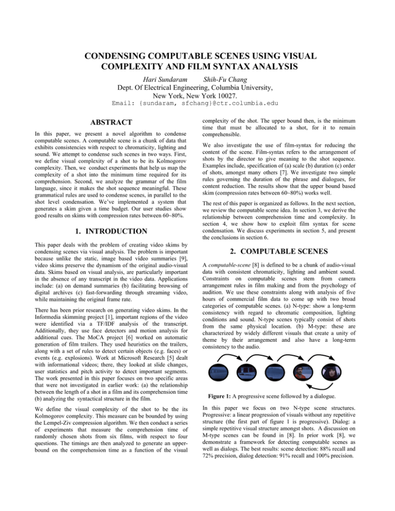
Figure 1: A progressive scene followed by a dialogue.
In this paper we focus on two N-type scene structures.
Progressive: a linear progression of visuals without any repetitive
structure (the first part of figure 1 is progressive). Dialog: a
simple repetitive visual structure amongst shots. A discussion on
M-type scenes can be found in [8]. In prior work [8], we
demonstrate a framework for detecting computable scenes as
well as dialogs. The best results: scene detection: 88% recall and
72% precision, dialog detection: 91% recall and 100% precision.
3. VISUAL COMPLEXITY
In this section, we discuss the relationship between visual
complexity of an image and its time for comprehension.
3.1 Insights: Film making and Human Learning
1
In film-making, there is a relationship between the size of the
shot and its apparent time (i.e. time perceived by the viewer).:
“Close-ups seem to last relatively longer on the screen than long
shots. The content of the close up is immediately identified and
understood. The long shot on the other hand, is usually filled
with detailed information which requires eye-scanning over the
entire tableau. The latter takes time to do, thus robbing it of
screen time” [7].
Recent results in experimental psychology [3] indicate the
existence of an empirical law: the subjective difficulty in
learning a concept is directly proportional to the Boolean
complexity of the concept (the shortest prepositional formula
representing the concept), i.e. to its logical incompressibility.
Clearly, there is empirical evidence to suggest a relationship
between visual “complexity” of a shot and its comprehensibility.
demonstrate how to map the normalized complexity (lLZ(X)/N)
of an image X to its comprehension time.
3.3 Complexity and Comprehension Time
We conducted our experiments over a corpus of over 3600 shots
from six films. A shot was chosen at random and then its keyframe presented to the subject (the first author). Representing
each shot by its key-frame is reasonable since our shot detection
algorithm [10], is sensitive to changes in color and motion. Then,
we measured the time to answer the following four questions (in
randomized order), in an interactive session: (a) who: [man
/woman/couple/people], (b) when: [morning/evening /afternoon],
(c) what: [any verb e.g. looking, walking], (d) where: [inside/
outside]3. The subject was expected to answer the questions in
minimum time and get all four answers right. This prevented the
subject from responding immediately. We conducted ten sessions
(to avoid fatigue), where the subject was questioned on 100 keyframes. In the end, we had the reaction times to 883 shots (we
averaged the reaction times over duplicates).
3.4 Analysis of Comprehension Time
3.2 Kolmogorov Complexity
We define the visual complexity of an shot to be its Kolmogorov
complexity. Let x be a finite length binary string of length n. Let
U(p) denote the output of an universal Turing machine2 U when
input with program p. Then:
KU ( x | n) !
min
p: U ( p ) = x
l ( p ),
Ub
Rayleigh bound
time
<1>
where, l(p) is the length of the program p, and n is the length of
the string x and where KU(x | n) is the Kolmogorov complexity of
x given n. Hence, the Kolmogorov complexity of x, with respect
to an universal Turing machine U is the length of the shortest
program that generates x. The Kolmogorov complexity of an
arbitrary string x is non-computable due to the non-existence of
an algorithm to solve the halting problem [2], [4]. Hence, we
must generate a reasonable upper bound on Kolmogorov
complexity. Lempel-Ziv encoding is a form of universal data
coding that doesn’t depend on the distribution of the source [2].
We can easily show the following lemma by using results in [2],
[4]. The proof has been omitted for the sake of brevity.
Lemma 1: Let {Xi} be a stationary, ergodic process over a finite
discrete sized alphabet. Let lLZ(X) be the Lempel-Ziv codeword
length of a string X, where X = {X1, X2, …, Xn}. Then,
KU ( X | n) ≤ lLZ ( X ) + c,
<2>
1
1
lim lLZ ( X ) → KU ( X | n).
n →∞ n
n
Hence, we can use the Lempel-Ziv compression algorithm to
upper bound the visual complexity of a shot. We now
Lb
Figure 2: Avg. comprehension time (sec.) vs. normalized
complexity (x-axis) showing comprehension (upper/lower)
bounds. It also shows the Rayleigh (95th percentile) bounds.
The histograms of the average comprehension time (i.e. the
average of the times to answer who? where? what? and when?)
obtained by discretizing the complexity axis, indicate that each
histogram slice is well modeled by a Rayleigh distribution. By
using the 95th percentile cut-off for each histogram we get an
estimate of the upper-bound on the comprehension time. The
lower-bound on the comprehension time is generated by
determining a least squares fit to the minimum time in each
histogram. The resulting bounds are shown in figure 2. The
equations for the lines are as follows:
U b (c ) = 2.40 c + 1.11,
Lb (c ) = 0.61c + 0.68,
<3>
where c is the normalized complexity and Ub and Lb are the
upper and lower bounds respectively, in sec. The lines were
1
The size (long/medium/close-up/extreme close-up) refers to the size of
the objects in the scene relative to the size of the image
2
An universal Turing machine U is a Turing machine that can imitate the
behavior of any other Turing machine T. It is a fundamental result that
such machines exist and can be constructed effectively [4].
3
Questions such as “How?” or “Why?” were not used in the experiment
since they cannot be answered by viewing just one image. Such questions
need an extended context (at least a few shots) for an answer.
estimated for c ∈ [0.25, 0.55] (since most of the data lies in this
range) and then extrapolated.
Hence, given a shot of duration to and normalized complexity cS,
we can condense it to at most Ub(cS) sec by removing the last to Ub(cS) sec. Let us assume that we want to reduce a sequence of
shots by 75%. Then, the target time for each shot is 25% of its
original length. If the target time of the shot is less than the upper
bound Ub for that shot, we use the upper bound. Shots that are
originally less than the upper bound are not reduced any further.
Note that equation <3> indicates that both the lower and upper
bounds increase with complexity, as they intuitively ought to.
The upper bound comprehension time is actually a conservative
bound. This is because of two reasons: (a) the shots in a scene in
a film are highly correlated (not i.i.d ) and (b) while watching a
film, there is no conscious attempt at understanding the scene.
4. FILM SYNTAX
In this section we shall give a brief overview of what constitutes
“film syntax.” Then, we shall discuss its utility in films and then
give time compression algorithms for two syntactic elements.
4.1 Defining Film Syntax
The phrase film syntax refers to the specific arrangement of shots
so as to bring out their mutual relationship [7]. In practice, this
takes on many forms (chapter 2, [7]) : (a) minimum number of
shots in a sequence (b) varying the shot duration, to direct
attention (c) changing the scale of the shot (there are “golden
ratios” concerning the distribution of scale) (d) the specific
ordering of the shots (this influences the meaning). These
syntactical rules lack a formal basis, but have been arrived at by
trial and error by film-makers. Hence, even though shots in a
scene only show a small portion of the entire setting at any one
time, the syntax allows the viewers to understand that these shots
belong to the same scene.
4.2 Why should we use Film Syntax?
Let us contrast shots with words in a written document. Words
have more or less fixed meanings and their position in a sentence
is driven by the grammar of that language. However, in films it is
the phrase (a sequence of shots) that is the fundamental semantic
unit. Each shot can have a multitude of meanings, that gets
clarified by its relationship to other shots. In the Informedia
project [1] the authors used object detectors (e.g. face detectors
etc.) to detect important shots; the audio was selected by a TFIDF analysis of the transcript and by selecting the complete
phrase surrounding the highly ranked words. An object detector
based approach (Informedia [1], MoCA [6]) to skims, for films,
at a conceptual level, makes the analogy “shots as words.”
However, this is in contrast to the way film-makers create a
scene, where the syntax provides the meaning of the shot
sequence. Hence, while condensing films, we must honor the
film syntax.
4.3 The Progressive Phrase
According to the rules of cinematic syntax, a phrase must have at
least three shots. “Two well chosen shots will create expectations
of the development of narrative; the third well-chosen shot will
resolve those expectations.” [7]. Let us assume that we have a
progressive scene that has k shots and is of duration Tp and
assume that we wish to reduce the duration by ∆tp. Then, we
have three cases (break points based on heuristics) to deal with.
k ≤ 6 : figure 3 (a) This contains only one major phrase. Hence,
we start with the last shot and keep dropping shots one shot at a
time, till either we have only three shots left or the scene
duration has been reduced by ∆tp.
6 < k < 15 : figure 3 (b) We assume that such a scene contains at
most two phrases. Then, we start removing shots from the middle
until the scene duration has been reduced by ∆tp or we are left
with the phrase at the beginning and at the end.
(a)
(b)
(c)
Figure 3: The black shots will not be dropped, and the
number of gray shots dropped will depend on ∆tp. The
arrows show the direction in which we start dropping shots.
k ≥ 15 : figure 3 (c) We assume that the scene contains at the
most three phrases. We start removing shots till we have the
phrase in the middle and the two end phrases or have reduced
time by ∆tp.
4.4 Dialogues
Figure 4: We start eliminating shots from the right.
Depicting a meaningful conversation between m people requires
at least 3m shots [7]. Hence in a dialogue that shows two
participants, this implies that we must have a minimum of six
shots. Let us assume that we have a dialogue scene that has k
shots and is of duration Td and assume that we wish to reduce the
duration by ∆td. The procedure for reducing dialogues is as
follows (figure 4): Start with the end of the dialogue and start
dropping shots till either we have six shots left or until we have
reduced the length of the dialogue by ∆td.
Note that reductions due to syntactical rules are at a different
level to the reductions due to visual complexity. The rules of film
syntax let us decide the number of shots to retain while
complexity analysis helps us determine the length of those shots.
5. EXPERIMENTS
The scenes used for creating the skims are from four films: Blade
Runner (bla), Bombay (bom), Farewell my Concubine (far), Four
Weddings and a Funeral (fou). The films were chosen since they
exhibit diversity in film-making styles. We arbitrarily used the
opening scene from each film for skim creation. We detect shots
using the algorithm to be found in chapter 2, [10].
We created an user interface
(figure 5) to specify target skim
length. The skim had to be
specified to use at least one of
the two reduction techniques:
(a) complexity reduction
(upper/lower bound) (c) syntax
reduction (yes/no).
The raw test scores as well as the “best/worst” classification by
the user (table 2) clearly indicate that the upper bound (Ub)
works well. The use of syntax has mixed results; while Ps and PsUb get high coherence scores, they are not consistently judged to
be the best (only 6/21). Ps-Lb has the maximum data reduction,
hence it is not surprising that it fares poorly.
Figure 5: The interface for
specifying the skim length.
The skims were of the
following types: (a) upper
bound (Ub) (b) lower bound (Lb) (c) pure syntax (Ps) (d) syntax
with upper bound (Ps-Ub) (e) syntax with lower bound (Ps-Lb).
Each skim represents a maximally reduced skim for that type
(table 1). Ub and Lb only use visual complexity, Ps uses syntax
only while other two use complexity and syntax based reduction.
Table 1: Skims lengths in seconds for each clip and skim type.
The numbers in brackets represent the percentage reduction. The
films in order: Blade Runner, Bombay, Farewell my Concubine,
Four Weddings and a Funeral.
Film Orig.
bla
bom
far
fou
184
114
153
165
Ub
Lb
Ps
44 (76)
45 (60)
53 (65)
31 (81)
21 (89)
21 (82)
26 (83)
14 (92)
114 (38)
41 (64)
103 (33)
58 (65)
Ps-Ub Ps-Lb
35 (81)
22 (81)
31 (80)
17 (90)
16 (91)
10 (91)
15 (90)
8 (95)
We conducted a pilot user study with five PhD students. The
study used four films (one clip from each), with five skims per
clip. Each clip had progressive and a dialog scene. The testers
were largely unfamiliar with the films (each film on the average
was familiar to 1.5 students) and were expected to evaluate the
skims on two metrics: (a) coherence: do the sequence of shots
tell a story? and (b) skip original?: confidence that having seen
the skim, there is no need to see the original. The metrics were
on a scale of 1-7 (strongly disagree = 1 and strongly agree = 7).
None of the clips or the skims had audio. We additionally asked
each tester to rate the “best” and the “worst” skim per clip. In
case of ambiguity, they could name more than one “best/worst”
skim.
Table 2: Test scores from five users. C: coherence, So: skip
original? The last two rows represent best/worst preferences.
Film
Ub
C
bla 5.8
bom 6.6
far 6.2
fou 6.0
all 6.15
best
9
worst
1
Lb
So
4.6
6.4
5.6
4.6
5.3
C
5.0
5.6
5.8
5.4
5.45
Ps
So
4.0
5.6
5.6
4.4
4.9
5
3
Ps-Ub
C
So
C
6.8 5.6 5.2
6.0 5.0 5.0
5.4 4.2 3.8
5.6 3.8 5.4
5.95 4.65 4.85
4
2
3
6
So
4.2
4.0
3.6
3.0
3.7
Ps-Lb
C
5.4
4.6
4.0
4.8
4.7
So
4.2
3.8
3.6
3.0
3.65
1
9
We showed the users a test clip and explained the two questions
of coherence and “skip original?” We then showed the original
clip, two skims, the original clip again and then followed by
three more skims. The original was shown first to establish a
context and then shown again in the middle of the test to refresh
the user. This procedure was repeated for the remaining three
clips. For each clip and each test taker, we randomized the order
of the skims. The results are shown in table 2.
6. CONCLUSIONS
In this paper, we’ve presented a novel framework for condensing
computable scenes. The solution has two parts: (a) visual
complexity and (b) film syntax analysis. We define the visual
complexity of a shot to be its Kolmogorov complexity. Then, we
showed how to effectively estimate this measure via the LempelZiv algorithm. Then we conducted an experiment that allowed us
to map visual complexity of a shot to its comprehension time.
The arrangement of shots in a scene gives meaning to the scene.
In this work, we devised algorithms based on simple rules
governing the length of the phrase and the dialog.
We conducted a pilot user study on four clips by using five
different skim types, each generated at maximal compression.
The results of the user study indicate that while all skims are
perceived as coherent (C>4.7) the upper bound based skim
(60~80% compression) works the best with the syntax based
summaries providing mixed results.
The algorithms presented here leave much room for
improvement: (a) we are working on incorporating audio into the
skims. (b) incorporating other elements of syntax such as scale
and time distribution of shots and differential changes in scale.
(c) we are conducting experiments to determine the robustness of
the proposed algorithm against different shot detection methods.
(d) additional experiments to verify the time-complexity curves
as well as a statistically significant user study (>25 students) are
also needed.
7. REFERENCES
[1]
M.G. Christel et. al Evolving Video Skims into Useful Multimedia
Abstractions, ACM CHI ′98, pp. 171-78, Los Angeles, CA, Apr.
1998.
[2] T.M. Cover, J.A. Thomas Elements of Information Theory, 1991,
John Wiley and Sons.
[3] J. Feldman Minimization of Boolean complexity in human concept
learning, Nature, pp. 630-633, vol. 407, Oct. 2000.
[4] M. Li, P. Vitányi An Introduction to Kolmogorov Complexity and
its Applications, 2nd ed 1997, Springer Verlag New York.
[5] H. Liwei et. al. Auto-Summarization of Audio-Video Presentations,
ACM MM ′99, Orlando FL, Nov. 1999.
[6] S. Pfeiffer et. al. Abstracting Digital Movies Automatically, J. of
Visual Communication and Image Representation, pp. 345-53, vol.
7, No. 4, Dec. 1996.
[7] S. Sharff The Elements of Cinema: Towards a Theory of Cinesthetic
Impact, 1982, Columbia University Press.
[8] H. Sundaram, Shih-Fu Chang Determining Computable Scenes in
Films and their Structures using Audio-Visual Memory Models,
ACM Multimedia 2000, pp. 95-104, Los Angeles, CA, Nov. 2000.
[9] S. Uchihashi et. al. Video Manga: Generating Semantically
Meaningful Video Summaries Proc. ACM Multimedia ′99, pp. 38392, Orlando FL, Nov. 1999.
[10] D. Zhong Segmentation, Indexing and Summarization of Digital
Video Content PhD Thesis, Dept. Of Electrical Engg. Columbia
Universty, NY, Jan. 2001.