Manifold Parameterization
Lei Zhang1,2 , Ligang Liu1,2‡ , Zhongping Ji1,2 , and Guojin Wang1,2
1
2
Department of Mathematics, Zhejiang University, Hangzhou 310027, China
State Key Lab of CAD&CG, Zhejiang University, Hangzhou 310027, China
‡
Correspondence: ligangliu@zju.edu.cn
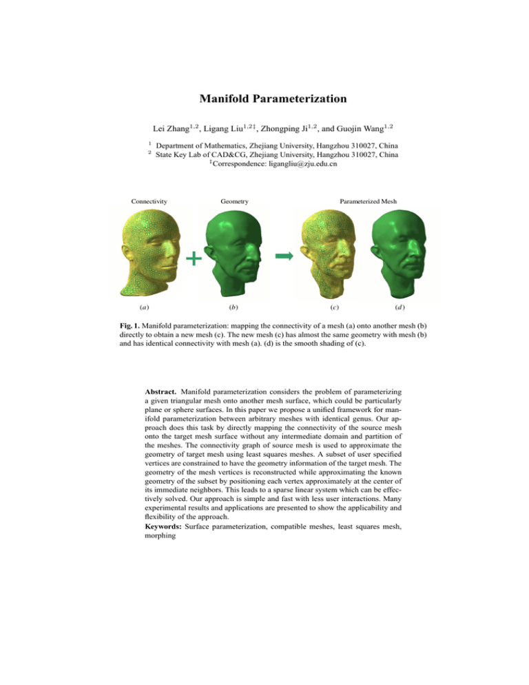
Connectivity
(a)
Geometry
(b )
Parameterized Mesh
(c )
(d )
Fig. 1. Manifold parameterization: mapping the connectivity of a mesh (a) onto another mesh (b)
directly to obtain a new mesh (c). The new mesh (c) has almost the same geometry with mesh (b)
and has identical connectivity with mesh (a). (d) is the smooth shading of (c).
Abstract. Manifold parameterization considers the problem of parameterizing
a given triangular mesh onto another mesh surface, which could be particularly
plane or sphere surfaces. In this paper we propose a unified framework for manifold parameterization between arbitrary meshes with identical genus. Our approach does this task by directly mapping the connectivity of the source mesh
onto the target mesh surface without any intermediate domain and partition of
the meshes. The connectivity graph of source mesh is used to approximate the
geometry of target mesh using least squares meshes. A subset of user specified
vertices are constrained to have the geometry information of the target mesh. The
geometry of the mesh vertices is reconstructed while approximating the known
geometry of the subset by positioning each vertex approximately at the center of
its immediate neighbors. This leads to a sparse linear system which can be effectively solved. Our approach is simple and fast with less user interactions. Many
experimental results and applications are presented to show the applicability and
flexibility of the approach.
Keywords: Surface parameterization, compatible meshes, least squares mesh,
morphing
1 Introduction
Surface parameterization can be viewed as a one-to-one mapping from a mesh surface
onto a suitable domain. There are lots of work on surface parameterizations in the literature [1]. Typically, surfaces that are homeomorphic to a disk are mapped onto the
plane. For closed genus-zero models, the unit sphere is a natural parameterization domain. More complicated mesh can be mapped to a coarse simplicial domain such as a
cube or its simplified mesh.
In general, the parameter domain itself will be a surface and so constructing a parameterization means mapping one surface onto another. This is widely used in applications such as shape morphing that require compatible meshes or consistent/cross
parameterization [2–4], i.e., meshes with identical connectivity.
In previous approaches, consistent parameterizations are generally constructed by
partitioning the meshes using a set of consistent cuts and creating an intermediate common domain [2–6]. There are many drawbacks for these approaches. It may require extra user input such as specifying the cut connectivity to partition two meshes into a set
of consistent patches. This is difficult for many models with dissimilar geometry. Furthermore, the mutual tessellation during optimization process is rather time-consuming
which makes it take a couple of hours to create inter-surface maps between two meshes.
Unlike previous approaches we try to directly create a one-to-one map between
topologically equivalent models. Our approach thinks of consistent parameterization
as embedding its connectivity graph onto another surface directly. We call it manifold
parameterization for the reason that manifold could refer to plane, sphere, and any other
manifold surface.
Our approach does this task by directly mapping the connectivity of one mesh onto
another mesh surface without any intermediate domain and partition of the meshes.
Considering Fig. 1 for an illustration example, in (c), the connectivity graph of the
mannequin head mesh (a) have been embedded on the surface of the Max-Planck head
mesh (b). Mesh (c) looks the same with mesh (b) in shape but has the same connectivity
with (a).
Our approach is rather intuitive and simple based on least squares meshes [7]. Using the same notations above, we use the connectivity of Ms by discarding its geometry
information. A subset of the vertices are then constrained to have the geometry information of Mt . The geometry of the mesh vertices is reconstructed in a least-square sense
while approximating the known geometry of the subset by positioning each vertex approximately at the center of its immediate neighbors [7]. This leads to a sparse linear
system which can be effectively solved. The location of each vertex in the subset is carefully chosen to be the features and saliency points of mesh Mt so that the reconstructed
surface captures the overall geometric shape of Mt . In this process, no any geometry
information of Ms is used. Since the reconstruction system accounts for both the given
connectivity of mesh Ms and the given geometry of mesh Mt , it yields a shape which
is a consistent parameterization between Ms and Mt .
To our knowledge, our approach is the first approach to directly generate the consistent parameterization between two manifold meshes without partitioning the meshes
using a set of consistent cuts and creating an intermediate common domain.
2 Related work
2.1 Mesh parameterizations
Planar parameterization methods established mappings between non-closed mesh and
planar domains. There have been many methods developed to date, see [1] for a recent
survey. An important limitation of planar parameterization techniques is that it generally
requires that an entire surface be cut into one or more disk-like charts, where each chart
is parameterized independently[8, 9].
A closed genus-zero surface can be parameterized into the unit sphere without any
cuts. Examples of spherical parameterization approaches include [10–12].
2.2 Consistent parameterizations
Consistent parameterizations have been done for morphing application in much of the
previous work, see a recent review on consistent parameterizations developed for morphing [13].
The typical approaches for consistent parameterization first parameterize the meshes
on a common base domain and then compute the overlapped triangulations on the based
domain. Sphere is chosen as a base domain for consistent parameterization in [14]. An
inherent limitation is that it can only be applied to closed, genus zero surfaces.
A more general approach is to parameterize the models over a common intermediate simplicial mesh [5, 2–4]. The meshes are partitioned into matching patches with
an identical inter-patch connectivity using a set of consistent cuts. Then each patch is
parameterized onto the corresponding face in the based domain.
The work of [5] first constructs simplicial parametrizations from two meshes to their
respective base domains. User assistance is required to form a good map between the
different domain meshes, and this map construction is not robust. The common metamesh is typically a reported 10 times more complex than either original mesh. A set
of genus-zero models is parameterized onto a simplicial complex in [2]. They create
consistent parameterizations by partitioning the mesh based on the connectivity of the
simplicial complex and parameterizing each patch onto the respective simplical complex face. The work of [3] improves the technique of [2] by not requiring the simplicial
complex to be specified a priori. However, their algorithm does not scale well with regard to the number of models to be consistently parameterized. In more recent work [4]
they construct consistent parameterizations between two models without going through
an intermediate domain. To generate a smooth consistent parameterization, they use a
symmetric, stretch based relaxation procedure, which trades high computational complexity for quality of the mapping. However the method is limited to dealing with only
two models and is very slow.
In this paper, we directly map the connectivity of one mesh onto another mesh
without any intermediate domain. Our approach needs not partition the meshes so that
no extra user inputs are required to specify the set of consistent cuts. Our system can
easily construct the consistent parameterization among multiple meshes as shown in
Section 5.1. Moreover, our approach is fast and efficient as it only needs to solve a
sparse linear system.
3 Least squares mesh
Least squares meshes (LS meshes) are meshes with a prescribed connectivity that approximate a set of control points in a least-squares sense [7]. For a given mesh connectivity, LS mesh allows that only a sparse subset of the mesh vertices contains geometric
information. The geometry of the mesh is reconstructed in a least squares sense by approximating the known geometry of the subset and positioning each vertex in the center
of gravity of its immediate neighbors. It can be obtained by solving a sparse linear system. The linear system not only defines a surface that approximates the given control
points, but it also distributes the vertices over the surface in a fair way.
We now go through the contexts of LS mesh quickly. For a vertex vi of mesh M ,
the following equation defines its smoothness condition:
vi −
X 1
vj = 0,
d
j∈i∗ i
(1)
where i∗ is the vertex index set of neighborhood vertices to the vertex vi and di is the
valence of vi .
It can be seen that the equations in Eq. 1 of all the vertices form a sparse linear
system. The linear system can be written in matrix form:
LX = 0,
(2)
where L is an n × n matrix, known as the Laplacian of the mesh, with elements as:

i = j,
 1,
Lij = − d1i , (i, j) ∈ E,

0,
otherwise,
X is the n × 1 column vector of the corresponding vertices. The above system had been
used in the planar graph drawing [15] and planar parameterization [16].
If the geometry of a subset of the vertices are provided, we can reconstruct the
geometry of the rest of the mesh vertices by solving the sparse linear system in Eq. 2
in a least square sense [7]. If we carefully select the provided vertices as feature points
of the surface, the reconstructed mesh can effectively approximate the original mesh.
Providing the 3D location for some s control vertices {vk = (xk , yk , zk )|k ∈ C},
where C = {i1 , i2 , . . . , is } is the set of indices. The system reconstructs the positions
of all the vertices v0 of mesh M to minimize the following error functional:
X
2
0 2
min
kLX
k
+
kvk0 − vk k .
(3)
0
X
k∈C
The above functional is quadratic in every vertex and hence its partial derivatives are
linear expressions. The unique minimum is found if all partial derivatives with respect
to the vertices vanish, which results in a sparse linear system as the following:
µ ¶
µ
¶
0
L
AX0 =
X0 =
= b,
(4)
F
bF
Connectivity
Geometry
(a)
(b )
(c )
(d )
( e)
Fig. 2. Manifold parameterization pipeline: mapping the connectivity of mannequin head model
(Ms ) onto David head model (Mt ). (a) Two head models (Upper: mannequin head; Lower: David
head) with user markers in blue; (b) LS mesh using the connectivity graph of mannequin head
mesh and user specified control points on the David head mesh; (c) Lower: the feature points
detected by mesh saliency approach [17] shown in pink; Upper: the detected feature points are
mapped onto (b) shown in green; (d) LS mesh using the connectivity graph of mannequin head
mesh and control points including user markers and mapped feature points on the upper mesh of
(c); (e) smooth shading of (d). The mesh (e) has the same geometry with David head model and
has the same connectivity with mannequin head model.
where F is an s × n matrix in which each row contains only one non-zero element used
to constrain the position of the control vertices with the element:
½
1, j = ik ∈ C,
fkj =
1 ≤ k ≤ s, 1 ≤ j ≤ n;
0, otherwise,
and bF is an s × 1 column vector:
bF
k = gik , 1 ≤ k ≤ s, g = x, y, or z.
Note that the linear system is defined for each component of the coordinates x, y,
and z. The positions of the vertices can be found by solving the sparse linear system in
Eq. 4 in a least square sense as:
X0 = (AT A)−1 AT b.
4 Our approach for manifold parameterization
4.1 Our approach
Inspired by LS meshes, we develop a new technique for manifold parameterization,
i.e., mapping the connectivity graph of one mesh onto another mesh. Given two man-
ifold meshes Ms and Mt , our goal is to generate a new mesh Mr which has the same
connectivity with Ms and the same geometry with Mt , as shown in Fig. 3.
Our strategy is to use the connectivity graph of Ms and use the constraints of control
points from Mt in the linear system Eq. 4. We need to carefully choose a set of control
points on Mt in order to bring the surface of Mr close to Mt .
Manifold parameterization
between M s and M t
=
Connectivity
of M s
+
Geometry
of M t
Fig. 3. Manifold parameterization: mapping the connectivity of Ms onto surface Mt .
4.2 User markers
Usually the consistent parameterization must respect the similar features between the
models. For example, when mapping between two human head models, the mouth must
map to the mouth, the nose to the nose, and so on. This is typically achieved by specifying the correspondence for a small set of feature vertices by the user, called user
markers, and using a consistent parameterization that preserves the user-defined feature
vertex correspondence.
In our system, the user can easily specify the corresponding marker points on two
given mesh shown side by side. Fig. 2(a) shows two mesh models, the mannequin
head mesh in the upper as Ms and the David head mesh in the lower as Mt , with user
specified corresponding feature points shown in blue.
4.3 Feature detection
The LS mesh M̄t constructed by the connectivity of Ms and the control points from the
user markers on Mt is shown in Fig. 2(b). It is seen in the figure that the LS mesh is
distorted and bears almost no similarities to the original shape of Mt due to the small
amount of control points.
Usually only a small number of marker paris is specified by the user. Thus we need
find more control points automatically to make the reconstructed M̄t get closer to the
shape of Mt .
Intuitively, the control points should be places in important locations where geometric detail is present on the surface, such as high curvature points, ridges and valleys,
and the tips of extruding parts.
In [17], the idea of mesh saliency is introduced as a measure of regional importance
for meshes, which is inspired by low-level human visual system cues. Mesh saliency
is defined in a scale-dependent manner using a center-surround operator on Gaussianweighted mean curvatures.
The pink points on David head mesh shown in lower row of Fig. 2(c) are the
detected feature points by approach of mesh saliency.
4.4 Mapping feature points
The feature points detected on mesh Mt should be mapped to the constructed mesh M̄t
so that M̄t can be reconstructed using these control points to get closer to the shape of
Mt .
We adopt an intuitive and simple method. Each vertex of the feature points on Mt
is mapped to the closet vertex on M̄t . Note that these closest points are required to be
the vertices M̄t .
It is required that the normals of the feature point on Mt and the corresponding
mapped point on M̄t should have compatible directions in the meaning of that their
inner product is larger than 0. This is to avoid mismatching so that front-facing surfaces
will not be matched to back-facing surfaces. The distance between the mapped pair
points is within a threshold and we use a distance threshold of 10% (measured as a
percentage of the bounding box diagonal) in our experiments.
There might be cases that multiple feature points on Mt are mapped onto one vertex
on M̄t . In these cases, we simply keep the closest pair and discard the other pairs.
It is also noted that simply mapping each feature point on Mt to its closest point on
M̄t will not always result in a very good matching as neighboring parts of Mt could get
mapped to disparate parts of M̄t . To constrain this problem, we use a heuristic criteria
by checking the normal changes in triangles related to mapped points over M̄t . Large
normal variation will penalize the point mapping. In our experimentation this method
can efficiently prevent adjacent parts of Mt from being mapped to disparate parts of M̄t .
As we will see in the following sections, the mismatching cases would seldom occur
for all testing examples after couples of iteration of LS mesh reconstruction as Mt and
M̄t are very close to each other.
To accelerate the minimum-distance matching, we use the ANN library [18] of approximating nearest neighbor searching, which performs quite efficiently in a linear
time.
The upper figure of Fig. 2(c) shows an example of this mapping. The feature points
(in pink color) on David head mesh shown in the lower figure of Fig. 2(c) are mapped
onto M̄t shown in Fig. 2(b). The mapped points on M̄t are shown in green in the
upper figure of Fig. 2(c). The mapped points are added into control points in LS mesh
construction and obtain the mesh M̄t shown in Fig. 2(d). It is seen that the reconstructed
mesh M̄t quickly gets closer to mesh Mt as the number of control points increases.
4.5 Algorithm steps
We summarize the steps of our approach as following:
Input: Two manifold triangular meshes Ms and Mt .
output: A consistent parameterization Mr between Ms and Mt .
Step 1. Specify some corresponding marker pairs on Ms and Mt manually.
Step 2. Detect the feature points with importance values on Mt by the approach of mesh
saliency.
Step 3. Construct M̄t by LS mesh using connectivity of Ms and markers’ geometry on
Mt as control points.
Step 4. Map the feature points of Mt onto M̄t .
Step 5. Construct M̄t by LS mesh approach using markers’ geometry and mapped
points’ geometry on Mt as control points.
Step 6. Perform adaptive refinements on M̄t and Ms simultaneously.
Step 7. Repeat Step 4 to Step 6 until the approximation error between M̄t and Mt is
within a prior tolerance. Then we get Mr = M̄t .
4.6 Discussion
At the first iteration, as M̄t is generated using only the user markers, the shape is much
different from Mt as shown in Fig. 2(b). Practically we do not use distance threshold
in the process of mapping feature points at the first iteration.
It can be seen that the connectivity of Ms should be dense enough to represent the
geometric details of Mt . Or else large distortion will occur. Although the adaptive refinement can alleviate this occasion, we usually subdivide/refine the mesh Ms at the
beginning to guarantee that there are enough triangles in its connectivity for some examples.
We would like to stress that the quality of the parameterization M̄t strongly depends on the shape of Ms and Mt and the specified marker pairs. In some cases the
connectivity of Ms is not dense enough to represent the geometry details of Mt globally or locally. In other case there will be skinny triangles on M̄t which cause numerical
problems in many applications. To account for this, we use two adaptive refinement operators, i.e., edge split and edge flip, to yield the parameterization M̄t representing the
geometry details of Mt with a better triangle shape.
A small quantity of feature points may be detected in some relatively smooth region
of Mt using the computed scale by mesh saliency approach. Then this region can not
be well approximated by LS mesh processing. Thus we select some random vertices in
this region and add these selected random vertices to the set of feature points generated
by mesh saliency.
Furthermore, our algorithm can be easily applied locally. Our system also allows to
consistently parameterized a part of a mesh less than another one, which happens to be
useful in practice.
5 Experimental results and applications
We will show some examples illustrating the applicability and flexibility of our manifold parameterization approach in a few exemplary applications. All the examples presented in this paper were made on a 2.8GHz Pentium IV computer with 1G memory.
5.1 Consistent parameterizations between multiple meshes
Our approach can be easily used to establishes parameterizations for a set of models. In
Fig. 4, the mannequin head model is parameterized on the other head models. After the
parameterizations, all the head models have identical connectivity with the mannequin
head model.
Connectivity
Geometry
Parameterized meshes
Fig. 4. Consistent parameterizations between multiple meshes: all the other head model are parameterized using the connectivity of the mannequin head model.
5.2 Spherical parameterization
As we have mentioned in previous sections, if the target mesh Mt has the geometry
of a plane, our approach can be regarded as an approach of planar parameterization; if
the target mesh Mt has the geometry of a sphere, our approach can be regarded as an
approach of spherical parameterization. Fig. 5 shows a spherical parameterization of
Venus head model by setting Mt as a sphere surface.
5.3 Mesh morphing
Establishing a one-to-one mapping between different shapes is the first step in morphing
application. Fig. 6 shows the use of the computed compatible meshes for morphing
between dinosaur and horse models. The morphing examples shown in Fig. 7 between
torus and mug demonstrates our approach’s ability to handle high genus models. Linear
interpolation is used in the above morphing examples. The accompany live video shows
the animation sequence of these morphing.
5.4 Texture transfer
Attributes from different models can be easily transferred through direct parametric
mapping if these models have the consistent parameterizations. Fig. 8 shows a simple
example of transferring texture. The texture of the tiger model is applied to the cheetah
model.
(a)
(b )
(c )
Fig. 5. Spherical paramterization of Venus head model. (a) Venus head mesh model; (b) the spherical parameterization of Venus head model; (c) smooth rendering the spherical parameterization
using the normal from original Venus head model.
Fig. 6. Morphing sequence between dinosaur and horse models.
Table 1 shows the statistics for the examples shown in the paper, including the vertex
number, the running time, and the Hausdorff distance [19] (with respect to the size of
bounding box). As we can see, our approach achieves a good combination of speed,
mesh quality, and shape preservation.
6 Conclusion
A unified manifold parameterization approach is presented in this paper. The connectivity of the source mesh is mapped onto another mesh surface directly without the
intermediate domain and specifying the consistent cuts. Our approach is based on the
least squares mesh. The geometry of the mesh vertices is reconstructed in a least-square
sense while approximating the known geometry of the subset by placing each vertex
approximately at the center of its 1-ring neighbors. Our approach provides a unified
framework for creating consistent parameterization between two manifold meshes with
higher (but same) genus if only a sufficient number of feature points are specified to
define a correspondence between the handles. Many experimental results have been
presented to show the applicability and flexibility of the approach.
The presented approach still has much to do for improvements and extensions. First,
our approach can not guarantee that all the vertices of parameterized mesh M̄t lie on
the surface of the target mesh Mt . A possible way to solve it might be combining with
Fig. 7. Morphing sequence between torus and mug models.
(a)
(b )
(c )
Fig. 8. Example of texture transfer. (a) A tiger model with textures; (b) a cheetah model; (c)
transferring texture of (a) onto (b).
Turk’s retiling approach [20]. Second, multiresolution solution could be integrated into
the framework to generate higher quality compatible triangulations between two much
dissimilar meshes. Last, it is also much worthwhile to extend our approach to generate consistent parameterization between manifold surfaces with different topologically
genus. We believe that this extension is feasible but not straightforward.
Acknowledgements
We would like to thank Zhonggui Chen for his help in video production. The textured tiger model used in Fig. 8 is courtesy of Dr. Kun Zhou from Microsoft Research
Asia. This work is supported by the National Natural Science Foundation of China (No.
60503067, 60333010), Zhejiang Provincial Natural Science Foundation of China (No.
Y105159) and the National Grand Fundamental Research 973 Program of China (No.
2002CB312101).
References
1. Floater, M.S., Hormann, K.: Surface parameterization: a tutorial and survey. In Dodgson,
N.A., Floater, M.S., Sabin, M.A., eds.: Advances in Multiresolution for Geometric Modelling. Springer-Verlag, Heidelberg (2005) 157–186
2. Praun, E., Sweldens, W., Schroder, P.: Consistent mesh parameterizations. In: Proceedings
of SIGGRAPH. (2001)
Table 1. Statistics including the vertex number, the running time, and the Hausdorff distance [19]
for the examples shown in the paper.
Model
Planck (Fig. 4)
Venus (Fig. 4)
David (Fig. 4)
Sphere (Fig. 5)
Horse (Fig. 6)
Mug (Fig. 7)
Cheetah (Fig. 8)
Vertex# Running Time(s)
10,139
91.5
10,139
108.1
10,139
133.3
8,628
12.8
10,189
10.8
38,400
82.5
22,192
172.4
Distance
0.0303
0.0051
0.057
0.0063
0.0091
0.0314
0.0105
3. Kraevoy, V., Sheffer, A.: Cross-parameterization and compatible remeshing of 3d models.
In: Proceedings of SIGGRAPH. (2004)
4. Schreiner, J., Asirvatham, A., Praun, E., Hoppe, H.: Inter-surface mapping. In: Proceedings
of SIGGRAPH. (2004)
5. Lee, A., Dobkin, D., Sweldens, W., Schrder, P.: Multiresolution mesh morphing. In: Proceedings of SIGGRAPH. (1999) 343–350
6. Lee, A., Sweldens, W., Schroder, P., Cowsar, L., Dobkin, D.: Maps: Multiresolution adaptive
parametrization of surfaces. In: Proceedings of SIGGRAPH. (1998) 95–104
7. Sorkine, O., Cohen-Or, D.: Least-squares meshes. In: Proceedings of Shape Modeling
International. (2004) 191–199
8. Gu, X., Gortler, S., Hoppe, H.: Geometry images. In: Proceedings of SIGGRAPH. (2002)
356–361
9. Sheffer, A.: Spanning tree seams for reducing parameterization distortion of triangulated
surfaces. In: Proceedings of Shape Modeling International. (2002) 61–66
10. Praun, E., Hoppe, H.: Spherical parameterization and remeshing. In: Proceedings of SIGGRAPH. (2003) 340–350
11. Gotsman, C., Gu, X., , Sheffer, A.: Fundamentals of spherical parameterization for 3d
meshes. In: Proceedings of SIGGRAPH. (2003) 358–364
12. Gu, X., Wang, Y., Chan, T.F., Thompson, P.M., Yau, S.T.: Genus zero surface conformal
mapping and its application to brain surface mapping. IEEE Transaction on Medical Imaging
23(7) (2004) 119–127
13. Alexa, M.: Recent advances in mesh morphing. Computer Graphics Forum 21(2) (2002)
173–196
14. Alexa, M.: Merging polyhedral shapes with scattered features. The Visual Computer 16(1)
(2000) 26–37
15. Tutte, W.T.: How to draw a graph. In: Proceedings of London Mathematical Society. (1963)
743–768
16. Floater, M.S.: Parameterization and smooth approximation of surface triangulations. Computer Aided Geometric Design 14(3) (1997) 231–250
17. Lee, C.H., Varshney, A., Jacobs, D.: Mesh saliency. In: Proceedings of SIGGRAPH. (2005)
18. Mount, D., Arya, S.: Ann: A library for approximate nearest neighbor searching (version
1.1). In: http://www.cs.umd.edu/ mount/ANN/. (2005)
19. Cignoni, P., Rocchini, C., Scopigno, R.: Metro: measuring error on simplified surfaces.
Computer Graphics Forum 17(2) (1998) 167–174
20. Turk, G.: Re-tiling polygonal surface. In: Proceedings of SIGGRAPH. (1992) 55–64