Detecting Image Near-Duplicate by Stochastic Attribute
Relational Graph Matching with Learning
Dong-Qing Zhang and Shih-Fu Chang
Department of Electrical Engineering,
Columbia University, New York, NY 10027.
{dqzhang,sfchang}@ee.columbia.edu
ABSTRACT
Detecting Image Near-Duplicate (IND) is an important problem in a variety of applications, such as copyright infringement detection and multimedia linking. Traditional image
similarity models are often difficult to identify IND due to
their inability to capture scene composition and semantics.
We present a part-based image similarity measure derived
from stochastic matching of Attribute Relational Graphs
that represent the compositional parts and part relations
of image scenes. Such a similarity model is fundamentally
different from traditional approaches using low-level features
or image alignment. The advantage of this model is its ability to accommodate spatial attribute relations and support
supervised and unsupervised learning from training data.
The experiments compare the presented model with several
prior similarity models, such as color histogram, local edge
descriptor, etc. The presented model outperforms the prior
approaches with large margin.
Keywords
Image Near-Duplicate Detection, Attribute Relational Graph
Matching, Part-based Image Similarity Measure
1. INTRODUCTION
Image Near-Duplicate (IND) refers to a pair of images in
which one is close to the exact duplicate of the other, but
different in the capturing conditions, times, rendering conditions, or editing operations. Detection and retrieval of
IND is very useful in a variety of real-world applications.
For example, in the context of copyright infringement detection, one can identify likely copyright violation by searching over the Internet for the unauthorized use of images.
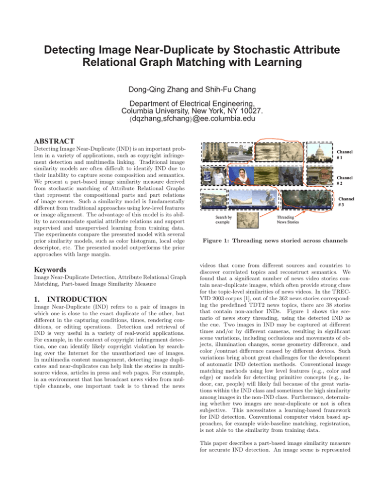
In multimedia content management, detecting image duplicates and near-duplicates can help link the stories in multisource videos, articles in press and web pages. For example,
in an environment that has broadcast news video from multiple channels, one important task is to thread the news
Channel
#1
Channel
#2
Channel
#3
Search by
example
Threading
News Stories
Figure 1: Threading news storied across channels
videos that come from different sources and countries to
discover correlated topics and reconstruct semantics. We
found that a significant number of news video stories contain near-duplicate images, which often provide strong clues
for the topic-level similarities of news videos. In the TRECVID 2003 corpus [1], out of the 362 news stories corresponding the predefined TDT2 news topics, there are 38 stories
that contain non-anchor INDs. Figure 1 shows the scenario of news story threading, using the detected IND as
the cue. Two images in IND may be captured at different
times and/or by different cameras, resulting in significant
scene variations, including occlusions and movements of objects, illumination changes, scene geometry difference, and
color /contrast difference caused by different devices. Such
variations bring about great challenges for the development
of automatic IND detection methods. Conventional image
matching methods using low level features (e.g., color and
edge) or models for detecting primitive concepts (e.g., indoor, car, people) will likely fail because of the great variations within the IND class and sometimes the high similarity
among images in the non-IND class. Furthermore, determining whether two images are near-duplicate or not is often
subjective. This necessitates a learning-based framework
for IND detection. Conventional computer vision based approaches, for example wide-baseline matching, registration,
is not able to the similarity from training data.
This paper describes a part-based image similarity measure
for accurate IND detection. An image scene is represented
by an Attribute Relational Graph (ARG) that models the
compositional parts as well as their relations of image scenes.
The similarity model is thereby derived from the likelihood
ratio of the stochastic transformation process that transforms one ARG to the other. Such a stochastic similarity model provides a principled framework for computing
similarity. More importantly, the stochastic model enables
the similarity measure to be learned from training data in
both supervised and unsupervised fashions. Intuitively, for
matching two images, this stochastic model characterizes a
scene transformation model that accommodates the variations of two near-duplicate images, including movements of
objects, occlusions and appearances of new objects.
We show that the approximate computation of the likelihood ratio can be realized by the well-known Loopy Belief
Propagation (LBP) algorithm. Fast LBP scheme is developed to speed up the likelihood computation. Learning of
the similarity model is carried out in the vertex-level with
supervised fashion and in the graph-level with unsupervised
manner using Expectation-Maximization.
To the best of our knowledge, this is the first statistical
framework that accommodates all types of variations of IND
and the first part-based image similarity model supporting
both supervised and unsupervised learning. The framework
is also general in the sense that more features of the image
can be easily incorporated.
The paper is organized as following: Section 2 presents the
prior work on image duplicate detection, image similarity
model and graph matching. Section 3 analyzes the variations of image near-duplicates in multimedia databases.
Section 4. presents the part-based representation for image scene, followed by Section 5. on matching Attribute
Relational Graph. Section 6. introduces camera model for
enhancing the baseline system. Section 7. describes the
experimental set-up and result analysis.
2. RELATED PRIOR WORK
Image Exact-Duplicate (IED) detection has been exploited
in various contexts. In [3][?], image and video copy detection was investigated using image similarity measure by lowlevel features, for instance, color histogram and local edge
descriptor. In contrast, rare work can be found on IND detection. The published work we can find is [7], the IND
detection is realized by global camera calibration, change
area detection and analysis of change area. The framework
is established in a rule-based manner and does not support
learning distance measure from training data.
Image similarity model has been studied for decades. Indexing by low-level features is an efficient technique, but lacks
the discriminative power for IND detection due to its inability to capture scene semantics and composition. Semantic
representation, such as the model vector system [11][9] could
be a promising technique for IND detection. However, the
limitations of the model vector system for IND detection are
two folds: the vector representation of concepts fails to capture spatial/attribute relations of individual concepts; Most
concept detectors require a large number of examples for
learning.
Part-based image similarity has been previously pursued using 2-D string [4] and composite region templates (CRTs)[13].
However string representation is difficult to accurately represent visual scenes with complicated visual features, while
region-based representation is sensitive to the errors of region segmentation. Part-based approaches have also been
used in object/scene recognition [5] and scene generative
model [8]. The approach in this paper differs from scene
generative models in the sense that we do not assume scene
models for individual scene categories.
Previous methods for attribute relational graph matching
are realized by energy minimization [6], relaxation [10] and
spectral method [12]. However, none of these prior work
provide framework for supervised and unsupervised learning
of the similarity measure from training data.
3.
DEFINITION AND ANALYSIS OF IMAGE
NEAR-DUPLICATE
The definition of Image Near-Duplicate has been previously
provided by [7]. The following definition also considers IND
generated by human editing and of computer generated images.
Definition 1. Image Near-Duplicate (IND) is a pair of images in which one is close to the exact duplicate of the other,
but differs slightly due to variations of capturing conditions
(camera, camera parameter, view angle, etc), acquisition
time, rendering conditions, or editing operations.
The above definition is not completely unambiguous. For
example, given two images taken from the same site at
slightly different time, one tends to consider them IND. But
such a decision may be ambiguous and greatly depends on
the context. For example, images of a site taken hours (or
even months) apart may have significant difference and will
not be considered IND. However, in some scenarios such
as broadcast news video, such ambiguity can be greatly reduced due to production conventions and typical user expectation. For example, IND showing visuals of the same
site/event in breaking news are normally recognizable without much controversy.
In addition, we do not distinguish IND from exact duplicates, as the latter refers to exactly identical data, detection
of which is not challenging. We aim at discrimination of
IND from different images, which will be referred to as nonduplicate images.
3.1
Variations of Duplicates
The variations of two near-duplicate images can be caused
by a few reasons, which can be categorized as: content
change, camera change and digitization process. Figure 2.
illustrates the causes of the variations of two near-duplicate
images.
In photos and videos, the variations of image near-duplicates
can be further categorized as follows[7]:
• Scene changes: movement and occlusion of foreground
Scene
Change
Camera Change
Figure 2: The generation of IND
objects, absence or presence of foreground objects, background change, post editing of images, etc.
• Camera parameter changes: camera view point change,
camera tilting, panning, zooming, etc.
• Photometric changes: change of exposure or lighting
condition, etc.
• Digitization changes: hue shift, contrast change,resolution
change, etc.
Different image sources may have different types of duplicate
variations. For example, for photos, variations are mostly
caused by camera parameter changes, because the photographers tend to take more than one pictures with different
camera settings so that they can select the best result later.
In contrast, in broadcast news videos, variations are often
caused by content change due to the time difference of capturing duplicate images. Figure 3 shows several IND examples illustrating a range of IND variations. The images are
extracted from TREC-VID 2003 news video corpus.
data for Topic Detection and Tracking (TDT) [2], a major
evaluation event in the field of natural language processing.
The TREC-VID2003 corpus is partitioned into two subsets,
the development set and the test set. The development set
consists of 2128 news stories according to the TDT2 story
segmentation ground truth. These news stories are grouped
by the TDT annotators into 28 topic clusters(Note not all
stories are labeled in TDT2). The ground truth of the 28
clusters cover 362 stories in the corpus. Among these 362
stories, at least 38 video stories are found to contain duplicate or near-duplicate frames. These stories are distributed
across 10 topics. Table 1 lists some examples of INDs with
their related topics.
Table 1: Examples of Duplicates in News Videos
Topic
# of Stories having Duplicates
India nuclear test
CNN: 1, ABC: 3
Jerusalem
CNN: 1, ABC: 1
Indonesia violence
CNN: 1, ABC: 2
GM Strike
CNN: 4, ABC: 5
School Shooting
CNN: 1, ABC: 1
To investigate the variations of INDs, we extract 150 IND
pairs from the TREC-VID 2003 video corpus. The following
table manifests the variations of the extracted IND pairs.
These IND images are also used as the benchmark data for
performance evaluation.
Table 2: Breakout of INDs in news videos over different types of variations
Obj Move
New Obj
Hue
75
64
24
Illuminance Camera Angle Camera Zoom
52
40
34
3.3
Figure 3: Different variations of IND in News Video
Databases (Top: content change, Mid: lighting
change, Bottom: camera change
3.2 A Case Study of Duplicates in News Videos
To show the usefulness of IND detection in the scenario of
news video analysis. We conducted a statistical study on the
distribution and variations of INDs in the TREC-VID 2003
video corpus[1]. The TREC-VID2003 corpus consists of
news videos from CNN headline and ABC world news from
January 1998 to June 1998. The closed captions and speech
transcripts of these videos were also used as the benchmark
IND Detection and Retrieval
Essentially, there are two types of problems related to IND:
IND retrieval, aims at finding all images that are duplicate
or near-duplicate to an input query image. The problem
arises in the context of copyright violation detection, and
query-by-example applications. IND detection aims at finding all duplicate image pairs given all possible pairs from
the image source. The detected INDs could be used to link
news stories and group them into threads.
IND detection is more difficult than IND retrieval. Because
for the latter case, a query image has been chosen by a user,
who usually has some belief that a near-duplicate image exists in the database. The retrieval task is considered successful if the target appears in the returned images within
certain search scope.
The difficulty of IND detection is due to the fact that as
the size of database increases, the number of duplicate pairs
generally increases in a linear speed, while the number of
non-duplicate pairs increases in a quadratic speed, leading
to the deterioration of the detection precision.
VCP
Figure 4: Interest point based ARGs
4. PART-BASED REPRESENTATION OF VISUAL SCENE
Part-based image representation aims at representing the visual scene by its compositional parts and relations of parts.
The parts could be regions or interest points. Mathematically, part-based representation can be realized by Attribute
Relational Graph (ARG), defined as following
Definition 2. An attribute relational graph is a triple G =
(V, E, A), where V is the vertex set , E is the edge set,
and A is the attribute set that contains unary attribute ai
attaching to each node ni ∈ V , and binary attribute aij
attaching to each edge ek = (ni , nj ) ∈ E.
The unary attributes of an ARG characterize the properties
of the individual parts, while the binary attributes signify
the part relations. Parts can be captured by two popular
fashions: using salient feature points, or using segmented
regions. Region based representation is sensitive to region
segmentation errors, therefore we use interest point based
approach in our system. The Figure 4 shows the ARGs
with interest point representation.
We detect the interest points by using the SUSAN corner
detector[14]. Each vertex ni of an ARG is attached with a
11-dimension feature vector yi : two components for spatial and vertical coordinates; three components for RGB
color; six components for Gabor wavelet features. The Gabor wavelet features are extracted using Gabor filter banks
with two scales and three orientations (with window size
13x13 and 25x25). Only magnitudes of the filter responses
are included in the feature vector, and phase features are
discarded. Each edge (ni , nj ) of an ARG is attached with
a 2-dimension feature vector yij that represents the spatial
coordinate differences of the two vertexes. Currently, fullyconnected graphs are used to capture all possible pairwise
relations of vertexes.
Figure 5: Stochastic Transformation Process for
ARG similarity
Let H denotes the binary random variable corresponding to
two hypotheses: H = 1, the target graph Gt is transformed
from the source grough Gs , namely the two images are nearduplicate; H = 0, the two images are non-duplicate. Let
Y s = {{Yis }; {Yijs }|i, j ≤ N } denotes the unary and binary
t
}|u, v ≤
features of the source graph Gs ; Y t = {{Yut }; {Yuv
M } the features of the target graph Gs . Then we have the
transform likelihood p(Y t |Y s , H = 1), and p(Y t |Y s , H =
0) respectively. The similarity between Gs and Gt is then
defined as the likelihood ratio
S(Gs , Gt ) =
5.1 Stochastic ARG Matching
p(Y t |Y s , H = 1)
p(Y t |Y s , H = 0)
(1)
An image pair is classified as IND, if S(Gs , Gt ) > λ. λ is
a threshold. Adjusting λ yields different detection precision
and recall. Note that in general N = M . We decompose
the transformation process p(Y t |Y s , H) into two steps. The
first step copies the vertexes from Gs to Gt , referred to as
vertex copy process (VCP). The second step transforms the
attributes of the copied vertexes, referred to as attribute
transformation process(ATP). This cascade stochastic process is visualized in Figure 5. The transformation process
requires an intermediate variable to specify the correspondences between the vertexes in Gs and Gt . We denote it
as X, referred to as correspondence matrix, a random 0-1
matrix taking value from χ = {0, 1}N ×M . xiu = 1 means
the ith vertex in Gs corresponds to the uth vertex in Gt .
This is visualized in the Figure 6. For the case of one-to-one
correspondences of vertexes in Gs and Gt , we need to have
the following constraints
xiu ≤ 1;
xiu ≤ 1
(2)
u
i
By introducing X, the transformation process then can be
factorized as following:
p(Y t |Y s , X, H)p(X|Y s , H)
(3)
p(Y t |Y s , H) =
X∈χ
5. SIMILARITY MEASURE OF ARGS
In order to match two ARGs, we use a stochastic process to
model the transformation from one ARG to the other. The
similarity is measured by the likelihood ratio of the stochastic transformation process. We refer such a definition of
data similarity as the transformation principle of similarity(TPS). For visual scenes, the referred stochastic process
characterizes a scene transformation model accommodating
the scene changes discussed above.
ATP
y1s 1
y
s
2
Gs
2
1
s
y13
s
y3 3
2
y1t
y 2t y13t
4
t
y3
3
Gt
0
1
0
0
1
0
0
0
0
0
1
0
X
Figure 6: Vertex correspondences of two ARGs and
the correspondence matrix
H
X
Ys
the ATP is fully factorized as
t
s
p(Y t |X, Y s , H) =
p(yuv
|xiu , xjv , yij
)
p(yut |xiu , yis )
iu,jv
Yt
We assume that the Attribute Transformation Process is
governed by Gaussian distributions with different parameters. Accordingly, we have conditional density functions for
unary attributes
Figure 7: The generative model for ARG matching
p(X|Y s , H) characterizes the VCP and p(Y t |Y s , X, H) represents the ATP. The transformation process is visualized
as the generative graphical model in Figure 7. In order to
satisfy the constraint Eq.(2), we let VCP be represented as
a Markov network or Markov Random Field (MRF) with
a two-node potential that ensures the one-to-one constraint
being satisfied. The MRF model is written as
1 ψiu,jv (xiu , xjv )
φh (xiu )
p(X|Y s , H = h) =
Z(h) iu,jv
iu
where Z(h) is the partition function. h ∈ {0, 1} is the hypothesis. Note here we use notations iu and jv as the indices
of the elements in the correspondence matrix X. For simplifying the model, we assume that X is independent on Y s
given H. The 2-node potential functions are defined as
ψiu,jv (0, 0) = ψiu,jv (0, 1) = ψiu,jv (1, 0) = 1,
ψiu,jv (1, 1) = 0, for i = j or u = v;
ψiu,jv (1, 1) = 1, otherwise
∀iu, jv
The last 2 equations above enforce the one-to-one correspondence constraints listed in Eq.(2).The 1-node potential
function is defined as
φ0 (0) = p0
φ0 (1) = q0 ;
φ1 (0) = p1
iu
p(yut |xiu = 1, yis ) = N (yis , Σ1 );
p(yut |xiu = 0, yis ) = N (yis , Σ0 )
And conditional density functions for binary attributes
t
s
s
|xiu = 1, xjv = 1, yij
) = N (yij
, Σ11 )
p(yuv
t
s
s
p(yuv
|(xiu ∩ xjv ) = 0, yij
) = N (yij
, Σ00 )
It is not difficult to show
the partition function can
N N that
M
i!qhi . For the efficient
be written as Z(h) =
i=1 i
i
learning and likelihood calculation, we use the asymptotic
approximation of Z(h) as specified in the following theorem
Theorem 1. Let N ≤ M . When N → ∞, and M − N <
∞ The log partition function log(Z(h)) tends to
(4)
N log(qh ) + λ
where λ is a constant written as
N
1
N
N
λ = lim
log
i!
N →∞ N
i
i
i=1
which can be approximately calculated numerically.
Proof of this theorem can be found in our technical report
[16].
For the ATP, we use naı̈ve Bayes assumption to let all unary
and binary features independent given Y s and H. Therefore
(6)
The parameters Σ1 ,Σ11 ,Σ0 ,Σ00 are learned from training
data.
5.2
Induced Markov Random Field
According to these setups, the term inside the equation (3)
can be written as
p(Y t |Y s , X, H = h)p(X|Y s , H = h)
1 t
s
=
ψiu,jv (xiu , xjv ; yij
, yuv
)
φh (xiu , yis , yut )
Z(h) ij,uv
ij
Where
s
t
t
s
(xiu , xjv ; yij
, yuv
) = ψiu,jv (xiu , xjv )p(yuv
|xiu , xjv , yij
)
ψiu,jv
φh (xij , yis , yut ) = φh (xiu )p(yut |xiu , yis )
Therefore, the transformation likelihood becomes
φ1 (1) = q1
where p0 , q0 , p1 , q1 controls the probability that the vertexes
in the source graph are copied to the target graph under hypothesis H = 0, H = 1. Due to the partition function, any
ph , qh with identical ratio ph /qh would result in the same
distribution. Therefore, we can set ph as 1, and let qh be
learned from training data.
(5)
p(Y t |Y s , H = h) = Z (Y t , Y s , h)/Z(h)
(7)
where
Z (Y t , Y s , h) =
x ij,uv
t
s
ψiu,jv
(xiu , xjv ; yij
, yuv
)
ij
t
φh (xiu , yis , yu
)
which in fact is the partition function of the following induced MRF, in which each of its vertexes corresponds to an
entry of the correspondence matrix X
p(X|Y s , Y t , H = h)
1
t
s
t
= t s
ψ
(xij , xuv ; yij
, yuv
)
φh (xiu , yis , yu
)
Z (Y , Y , h) ij,uv iu,jv
ij
The partition function Z(h) can be approximately computed
from Eq.(4). The following section provides the approximate
computation scheme for Z (Y t , Y s , h).
5.3
Computation of the Likelihood
The computation of the exact induced partition function
Z (Y t , Y s , h) is intractable, since we have to sum over all
possible X in the set χ, whose cardinality grows exponentially with respect to N M . Therefore we have to compute
the likelihood using certain approximation.
5.3.1
Approximation of the Exact Likelihood
By applying the Jensen’s inequality on the log partition
logZ (Y t , Y s , h), we can find its variational lower bound as
following (more details can be found in [16]). The lower
bound then can be used as the approximation of the exact
likelihood
s
t
q̂(xiu , xjv ) log ψiu,jv
(xiu , xjv ; yij
, yuv
)
logZ ≥
M Step: Maximize the lower bound in Eq.(8) by varying
parameters. This can be realized by differentiating the lower
bound with respect to the parameters, resulting in the following update equations
iu,jv
+
q̂(xiu ) log φh (xiu , yis , yut ) + H(q̂(X)) (8)
iu
where q̂(xiu ) and q̂(xiu , xjv ) are approximate one-node and
two-node marginals, also known as beliefs. H(q̂(X)) is the
entropy of q̂(X), which does not have tractable decomposition for loopy graphical model. H(q̂(X)) can be approximated using Bethe/Kikuchi approximation [15], by which
[15] has shown that the q̂(xiu ) and q̂(xiu , xjv ) can be obtained by a set of fixed point equations, known as Loopy
Belief Propagation. The equation of the approximated entropy can be found in [15].
5.3.2
Fast Loopy Belief Propagation
The speed bottleneck of this algorithm is the Loopy Belief Propagation.
Without
any speedup, the complexity of
BP is O (N × M )3 , which is formidable for computation.
However, for complete graph, the complexity of BP can be
reduced by introducing an auxiliary variable. The BP message update rule is modified as follows
(t+1)
miu,jv (xjv ) = k
(t+1)
Miu
xiu
(t)
(t)
ψiu,jv (xiu , xjv )φh (xiu )Miu (xiu )/mjv,iu (xiu )
(t+1)
(xiu ) = exp Σkw=iu log(mkw,iu (xiu ))
Where Miu is the introduced auxiliary variable,
t is the it-
eration index. This modification results in O (N × M )2
computation complexity.
To further speed up the likelihood computation, early determination of the node correspondences (i.e.xiu ) can be realized by thresholding the one-node probability in the Eq.
(5). For example, if the coordinate of a vertex i in the source
graph deviate too much from the coordinate of the vertex
u in the target graph, the state variable xiu can be fixed
to zero with probability one. This operation is equivalent
to reduce the vertex number of the induced MRF model,
resulting in less computation cost.
5.4 Learning the Parameters
Learning ARG matching can be performed at two levels:
vertex-level and graph-level. For the vertex level, the annotators annotate the correspondence of every vertex pair.
This process is very expensive, since typically one image
includes 50-200 interest points. In order to reduce human
supervision, graph-level learning can be used, where annotators only indicate whether two images are IND or not without identifying specific corresponding interest points .
For learning at the vertex-level, maximum likelihood estimation results in the direct calculation of the mean and variance of Gaussian functions in the Eq.(5)(6) from the training
data. The resulting estimates of the parameters are thereby
used as the initial parameters for the graph-level learning.
For learning at the graph-level, we can use the following
variational Expectation-Maximization (E-M) scheme:
E Step: Compute q̂(xiu ) and q̂(xiu , xjv ) using Loopy Belief
Propagation.
ξiu
=
Σ1
=
Σ0
=
Σ11
=
Σ00
=
q̂(xiu = 1); ξiu,jv = q̂(xiu = 1, xjv = 1)
t
s
t
s T
k
iu (yu − yi )(yu − yi ) ξiu
ξ
k
iu iu
t
s
t
s T
k
iu (yu − yi )(yu − yi ) (1 − ξiu )
k
iu (1 − ξiu )
t − y s )(y t − y s )T ξ
(y
iu,jv
uv
uv
k
iu,jv
ij
ij
ξ
k
iu,jv iu,jv
t − y s )(y t − y s )T (1 − ξ
(y
iu,jv )
uv
uv
k
iu,jv
ij
ij
(1
−
ξ
)
iu,jv
k
iu,jv
Where k is the index for the instances of the training graph
pairs.
For the prior parameter qh , the larger ratio q1 /q0 would
result in the more contribution of the prior model to the
overall transformation likelihood ratio. Currently, we use a
gradient descent scheme to gradually increase the value of
q1 (start from 1) until we achieve the optimal discrimination
of IND classification in the training data. More details can
be found in [16].
6.
CAMERA TRANSFORMATION
Camera change may result in significant interest point movements, resulting in low matching likelihood. Therefore, we
exploit to use camera parameter estimation and calibration
to avoid the mismatch if two scenes are nearly identical but
are captured by different camera settings.
Two images captured by different camera parameters are
coupled by multi-view geometry constraints. There are essentially two types of constraints: homography and fundamental matrix. Basically, homography transform captures
the viewing direction change of the camera, while fundamental matrix captures other types of camera parameter
changes. In the current project, we only implemented the
homography transform.
Under homography constraint, one interest point in the source
image, described by the homogenous coordinate vector X1 =
(T x1 , T y1 , T ) is mapped to one point X2 = (T x2 , T y2 , T )
in the target image by the homography transform H:
X2 = HX1
(9)
Here we use the vertex matching results yielded by the
Loopy Belief Propagation. That is, if xiu > 0.5, then we
consider the interest point i and u correspondent. After
the estimation of the homography, the spatial attributes in
the source ARG are calibrated by applying the estimated
homography matrix.
7.
EXPERIMENTS AND RESULTS
The benchmark data are collected from the TREC-VID 2003
corpus. The data set consists of 150 IND pairs (300 images)
and 300 non-duplicate images. 100 IND pairs and all 300
non-duplicate images are from the keyframe set provided by
the TREC-VID 2003, while the remaining 50 IND pairs are
non-keyframes. The entire data set is partitioned into the
1
training set and the testing set. The training set consists of
30 IND pairs and 60 non-duplicate images.
0.8
7.1 Implementation Issues
0.7
0.6
Precision
From the approximate likelihood equations, we observe that
the likelihood ratio is not invariant to the sizes of the input
graphs. To reduce the sensitivity of the size variation. We
use the averaged likelihood ratio S(Gs , Gt )/(M N ) instead
of S(Gs , Gt ). Furthermore, we assume that under negative hypothesis H = 0, there is no vertex correspondence
between Gs and Gt . Therefore, all xiu and xiu,jv are set
to 0 with probability 1. And the Gaussian parameters for
H = 0 are the same as those for H = 1. To reduce the
computational cost, we use the early determination scheme
by a thresholding process. As a result, the maximum size
of the induced MRF is 150 vertexes. The average computation time of matching two images is about 0.4 second. The
speed may be further boosted using more sophisticated fast
BP schemes, as recently studied by some researchers.
GRAPH
GRAPH−M
AFDIP
CH
LED
0.9
0.5
0.4
0.3
0.2
0.1
0
0.1
0.2
0.3
0.4
Recall
0.5
0.6
0.7
0.8
Figure 8: The performance comparison with the
previous approaches and ARG matching without inference and learning
7.2 Learning Procedure
7.3 Performance Comparison with Previous
Methods
The performance of the developed method (GRAPH) is compared with color histogram (CH), local edge descriptor (LED),
averaged features distance of interest points (AFDIP) and
graph matching with manual parameter setting (GRAPHM). Local edge descriptor has been demonstrated as the
best feature for image copy detection in the previous work
[?]. For color histogram, we use HSV color space with 64
bins of H, 8 bins of S, and 4 bins of V. AFDIP is the summation of all possible cosine distances between the unary
feature vectors of the interest points in Gs and Gt divided
by N M . GRAPH-M is the graph matching likelihood ratio
under the manually selected Guassian parameters. The parameters are obtained by manually adjusting the covariance
matrices until we observe the best interest point matching
results (by binarizing the belief q̂(xiu )). The parameters are
initialized using vertex-level learning with two IND pairs.
recall is defined as the number of the correctly detected IND
pairs divided by the number of all ground truth IND pairs.
Precision is defined as the number of the correctly detected
IND pairs divided by the number of all detected IND pairs.
From the results, we observe that the averaged feature distance performs even worse than color histogram while graph
matching with training performs best. This indicates that
the performance of graph matching mainly gains from the
probabilistic inference and learning. Graph matching with
learning also outperforms graph matching with manual parameter setting. This confirms that the learning process
not only reduces the human labor cost but also significantly
improves the performance by capturing data statistics.
7.4
Sensitivity to Interest Point Detection
We study if the algorithm is sensitive to the interest point
detection. The algorithm is applied with different parameters of the corner detection algorithm (GRAPH, GRAPHL, GRAPH-S), resulting in different numbers of the interest
points and slight changes of their locations. The Figure 9
shows that the sensitivity to the interest point detection is
fairly low comparing with the performance variation across
different methodologies. This demonstrates the robustness
of our method by using interest point based representation.
1
GRAPH
GRAPH−L
GRAPH−S
CH
0.9
0.8
0.7
0.6
Precision
Learning process consists of two phases. In the first phase,
we apply the supervised vertex-level learning, where the correspondences of interest points are marked by the annotator.
The number of interest points varies from 50 to 200 per image. Only 5 near-duplicate pairs and 5 non-duplicate pairs
are used in vertex-level learning. In the second phase, we
conduct the graph-level learning. E-M scheme is carried out
using 25 IND pairs and 25 Non-IND pairs.
0.5
0.4
0.3
0.2
0.1
0
0.1
0.2
0.3
0.4
Recall
0.5
0.6
0.7
0.8
Figure 9: Study of sensitivity to different interest
point detection parameters
7.5
Does Camera Transformation Help?
To see if the inclusion of the camera transform model indeed
helps IND detection, we compare the performance of the system with camera transform and without camera transform.
The results show that camera transform only contributes little performance improvement. This is likely due to inaccurate camera parameter estimation, since most INDs involve
substantial content change. This again confirms that detecting IND in such a domain is challenging for the conventional
image registration approaches.
8.
1
GRAPH
GRAPH+CAM
0.9
0.8
0.7
0.6
Precision
CONCLUSIONS
We present a novel part-based image similarity measure by a
learning-based matching of attribute relational graphs that
represent images by their parts and part relations. Such
a similarity model is fundamentally different from the conventional ones using low-level features or registrations. We
show that the presented similarity measure outperforms previous approaches with large margin in detecting Image NearDuplicate. The experiments also show that the similarity
measure is insensitive to the parameter settings of interest
point detection, and camera models contribute little performance improvement.
0.5
0.4
0.3
0.2
0.1
0.1
0.2
0.3
0.4
Recall
0.5
0.6
9.
0.7
REFERENCES
[1] http://www-nlpir.nist.gov/projects/trecvid/. Web site,
2004.
Figure 10: Study the performance gain by the inclusion of camera model
[2] J. Allan, J. Carbonell, G. Doddington, J. Yamron, and
Y. Yang. Topic detection and tracking pilot study: Final
report. In Proceedings of the DARPA Broadcast News
Transcription and Understanding Workshop, 1998., 1998.
7.6 Duplicate Retrieval
[3] E. Chang, J.Wang, C.Li, and G. Wiederhold. Rime: A
replicated image detector for the world wide web. In
Proceedings of SPIE Mulimedia Storage and Archiving
Systems III. IEEE, Nov. 1998.
Retrieval problem is important for some applications, such
as copyright violation detection. Let Qc denotes the number of queries that correctly retrieve its duplicate version in
the top K retrieved images. Let Q denotes the overall number of queries. Then the retrieval performance is defined
as P (K) = Qc /Q, the probability of the successful top-K
retrieval. In the current experiment, for each query image,
we know there is one and only one duplicate version in the
database.
As shown in the Figure 11, the graph matching approach
outperforms others when K ≤ 50. However, when K is
larger than 50 (although in practice, users typically do not
view more than 50 results), the performance of graph matching is lower than that of the color histogram. This is primarily because the likelihood ratio of graph matching quickly
decays to nearly zero when two images are not matched. As
a result, the ranks of these likelihood ratios become inaccurate. We also observed that the color histogram retrieved
90% duplicates when K ≥ 100. This indicates that low cost
approaches like color histogram can be used as a prefilterring step to narrow down the search scope, in which the
more accurate graph matching method can be applied.
0.6
P(K) : Probability of sucessful retrieval
[5] R. Fergus, P. Perona, and A. Zisserman. Object class
recognition by unsupervised scale-invariant learning. In
Proceedings of the IEEE Computer Vision and Pattern
Recognition Conference, pages 66–73. IEEE, 2003.
[6] H.G.Barrow and R. Popplestone. Relational descriptions in
picture processing. Machine Intelligence, 6:377–396, 1971.
[7] A. Jaimes. Conceptual structures and computational
methods for indexing and organization of visual
information. Ph.D. Thesis , Department of Electrical
Engineering, Columbia University, February 2003.
[8] N. Jojic, N. Petrovic, and T. Huang. Scene generative
models for adaptive video fast forward. In International
Conference on Image Processing (ICIP), Barcelona, Spain,
2003. IEEE, 2003.
[9] C.-Y. Lin, B. L. Tseng, M. Naphade, A. Natsev, and J. R.
Smith. Videoal: A novel end-to-end mpeg-7 automatic
labeling system. In IEEE Intl. Conf. on Image Processing
(ICIP). IEEE, September 2003.
[10] R.C.Wilson and E.R.Hancock. Structual matching by
discrete relaxation. IEEE Trans. Pattern Anal. Mach.
Intell., 19:1–2, 1997.
[11] J. R.Smith, M. Naphade, and A. Natsev. Multimedia
semantic indexing using model vectors. In IEEE Intl. Conf.
on Multimedia and Expo (ICME). IEEE, 2003.
0.7
[12] J. Shi and J. Malik. Self inducing relational distance and
its application to image segmentation. Lecture Notes in
Computer Science, 1406:528, 1998.
0.5
0.4
[13] J. R. Smith and C.-S. Li. Image classi cation and querying
using composite region templates. Journal of Computer
Vision and Image Understanding, 2000.
0.3
0.2
[14] S. Smith. A new class of corner finder. In Proc. 3rd British
Machine Vision Conference, pages 139–148, 1992.
GRAPH
GRAPH−M
CH
AFDIP
LED
0.1
0
[4] S.-K. Chang. Principles of pictorial information systems
design. Prentice-Hall, Inc., 1989.
5
10
15
K : search scope
20
25
Figure 11: IND retrieval performance
30
[15] J. S. Yedidia and W. T. Freeman. Understanding belief
propagation and its generalizations. In Exploring Artificial
Intelligence in the New Millennium, pages Chap. 8, pp.
239–236, January 2003.
[16] D.-Q. Zhang and S.-F. Chang. Stochastic attribute
relational graph matching for image near-duplicate
detection. DVMM Techinical Report, Dept. of E.E.,
Columbia University, July 2004.