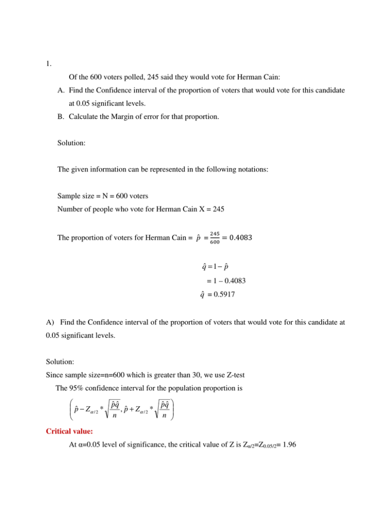
1.
Of the 600 voters polled, 245 said they would vote for Herman Cain:
A. Find the Confidence interval of the proportion of voters that would vote for this candidate
at 0.05 significant levels.
B. Calculate the Margin of error for that proportion.
Solution:
The given information can be represented in the following notations:
Sample size = N = 600 voters
Number of people who vote for Herman Cain X = 245
The proportion of voters for Herman Cain = p̂ =
0.4083
qˆ = 1 − pˆ
= 1 – 0.4083
q̂ = 0.5917
A) Find the Confidence interval of the proportion of voters that would vote for this candidate at
0.05 significant levels.
Solution:
Since sample size=n=600 which is greater than 30, we use Z-test
The 95% confidence interval for the population proportion is

 pˆ − Zα / 2 *


pˆ qˆ
, pˆ + Zα / 2 *
n
pˆ qˆ 

n 
Critical value:
At α=0.05 level of significance, the critical value of Z is Zα/2=Z0.05/2= 1.96
By substituting the values in the above formula we get,

0.41 * 0.59
0.41 * 0.59 
 0.41 − 1.96 *

,
0
.
41
+
1
.
96
*


600
600


(0.41 − 1.96 * 0.020079,0.41 + 1.96 * 0.020079)
(0.41 − 0.03935,0.41 + 0.03935)
(0.369, 0.447)
Hence 95% confidence interval estimate of the proportion of votes is (37%, 45%).
/---------------------------/
Calculate the Margin of error for that proportion.
Solution:
Margin of Error: E = Zα / 2 *
E = 1.96 *
pˆ qˆ
n
0.41* 0.59
600
Therefore, the margin of error for the given proportion is 0.020079.
/---------------------/
Problem: 2
The data below represents the ages of undergraduate students at Harper College and Daley
College. Use the information to answer questions 27 to 29.
Harper:
Daley College
Number Sampled = 14
Number = 12
Mean = 21
Mean = 22
Standard Dev = 2.5
SD = 2.8
1.
Perform the requested operation:
C. Find the Critical Value of t to test the claim that the ages of students in the two colleges
are similar at 0.05 significant levels.
D. Calculate the Confidence interval of the Mean for Harper College students
Solution:
C)
At α = 0.05 level of significance, the critical value of t with (n1+n2-2) =24 degrees of
freedom is given by
tα / 2, n −1 = t0.025, 24 df = 2.3909
(by referring t-distribution table)
By substituting the values in the above formula we get,
/----------------/
d) The 95% confidence interval for the difference between the two population means is given by

s2 s2
( X 1 − X 2 ) − t0.025 * 1 + 2 ,
n1 n2

( X 1 − X 2 ) + t0.025 *
s12 s22 
+ 
n1 n2 
From the above table, we have

2.52 2.82
2.52 2.82 
+
, (21 − 22) + 2.3909 *
+
(21 − 22) − 2.3909 *

14
12
14
12 

[–3.507, 1.507]
Thus, the 95% confidence interval for the difference between the two population means is
[–3.507, 1.507].
/---------------------/
3. Perform the requested operation:
A. Find the Critical Value of F to test the claim that the ages of students in the two colleges
are similar at 0.05 Significant level.
B. Calculate the Coefficient of variation for the two groups and interpret them
Solution:
A. The Critical value of F is given by, F0.05, 14,12 = 2.64 (by referring F-table)
B. The coefficient of variation is a calculation built on other calculations -- the
standard deviation and the mean -- as follows:
C.V = 11.90
Problem: 4
In a clinical experiment, a researcher wants to test the effect of Medical Marijuana on Glaucoma
patients. He conducts a double-blind study using marijuana and a placebo (fake weed). The table
below summarizes the data on patient response of ‘feeling better’. With 95% Confidence, should
medical marijuana be recommended?
Questions
correctly
answered Questions answered correctly
Placebo Group
n = 42
Mean = 43.14
SD = 7.74
Marijuana Group
n = 34
Mean = 40.76
Var = 61.15
Solution:
The given information can be represented in the following notations:
Sample size of Placebo Group = n1 = 42
Sample size Marijuana Group = n2 = 34
Sample mean of Placebo Group = X 1 = 43.14
Sample mean of Marijuana Group = X 21 = 40.76
Sample standard deviation = S1 = 7.74
Sample standard deviation = S2 = 7.82
Hypotheses:
Null hypothesis: H0 : With 95% Confidence, medical marijuana can be recommended.
Alternate hypothesis: H1 : With 95% Confidence, should medical marijuana cannot be
recommended.
Using Microsoft addins called Megastat we get,
Hypothesis Test: Independent Groups (z-test)
Placebo Group
42
7.74
43
Marijunana Group
34
7.82
41
8.000
1.698
0
4.71
2.47E-06
4.671
11.329
3.329
mean
std. dev.
n
difference (Placebo Group - Marijunana Group)
standard error of difference
hypothesized difference
z
p-value (two-tailed)
confidence interval 95.% lower
confidence interval 95.% upper
half-width
F-test for equality of variance
61.1524
59.9076
1.02
.9458
variance: Marijunana Group
variance: Placebo Group
F
p-value
Conclusion:
Since the P-value (0.9458) corresponding to the value of test statistic (4.71) is greater than 0.05,
there is sufficient evidence to accept the null hypotheses at 5% level. Hence we conclude
medical marijuana can be recommended.
Procedure:
Problem: 5
A researcher wants to know if the Race and having a Single parent has an factor on gun violence
in a small town. A small group of that town residents were surveyed on their experience with
violence involving a family member. The computer printout of the ANOVA table below
summarizes the results. Interpret your results.
Two-Way ANALYSIS OF VARIANCE
Source
Sum of
Squares
Degrees of
freedom
Mean
square
F-ratio
Significance
of F
Race
Single parent
Interaction
Residue
10.00
0.42
0.41
3.17
1
1
1
6
10.00
0.42
0.41
0.53
18.87
0.79
0.77
0.03
.40
.41
Total
14
9
A. Interpret your results using the classical approach (F-value only)
B. Using
α = 0.05, interpret your results using the p-value approach (p-value and alpha)
Solution:
a)
From the above table, we have
The p-value of the main effect Race is 0.03
The p-value of the main effect Single Parent is 0.40
The p-value of the interaction is 0.41
b)
Conclusion:
Since the p-value of the main effect Race is less than 0.05, we reject the null hypothesis
at 0.05 level of significance. Hence we conclude that at least two population means differ
significantly among the levels of the factor Race
Since the p-value of the main effect Single Parent is greater than 0.05, we do not reject
the null hypothesis at 0.05 level of significance. Hence we conclude that there is no significant
difference in population means among the levels of the factor Single Parent
Since the p-value of the interaction effect Race and Single Parent is greater than 0.05, we
do not reject the null hypothesis at 0.05 level of significance. Hence we conclude that there is no
significant difference in the interaction between the factors Race and Single Parent.
/-----------------------/
29. Perform the requested operations:
(10 points)
a. Before a student takes a Statistics prep class, he or she must take a pretest and then a posttest
after the completion of the course. Typical results for two students are shown in the table
below.
Pretest
510
475
Posttest
662
620
i. Which is the independent variable?
ii. Write an equation that models the test scores
iii. Interpret the model
Solution:
(i)
(ii)
Pretest is the independent variable, because pretest is taken before completion of
the course
Pretest Vs Posttest
665
y = 1.2x + 50
R² = 1
660
655
Posttest
650
645
640
635
630
625
620
615
470
480
490
500
510
520
Pretest
(iii)
As the X-values increases the Y value also increase using regression equation.
/----------------------/
b. The cost of one day car rental is the sum of the rental fee, $100, plus $.78 per mile.
i. Write an equation that models the cost associated with renting a car.
Solution:
Y =. $78x + $100
ii. Interpret the model
Solution:
As the number of miles increase the rental cost of the car also increases.
iii. Find the cost of renting a car and driving it for 1000 miles.
Solution:
Y =. $78x + $100
Y =. $78(1000) + $100
Y = $880
Therefore, the cost of renting a car and driving it for 1000 miles is $880.
30. Administrators wanted to predict a students grade on a Senior College Statistics Midterm
based on his/her SAT score. A sample of ten past senior students was selected and their
recorded SAT scores and Midterm scores listed. The table below summarizes that data.
(15 points)
Student
ID
AB
CD
EF
GH
IJ
LM
NO
PQ
RS
TZ
•
SAT score
(Independent Variable) x
1100
1300
1000
1100
1200
1200
1400
1300
1000
1400
Midterm
score
(Dependent Variable) y
89
92
86
92
90
93
98
95
88
95
Use your calculator or statistical software to sketch the scatter plot for this data
and determine the correlation coefficient (r) between SAT and Midterm scores.
Solution:
SAT score (x) VS SAT score (y)
100
98
y = 0.022x + 65.4
R² = 0.809
SAT Score (y)
96
94
92
90
88
86
84
500
700
900
1100
SAT Score (x)
1300
1500
•
With α = 0.05, test the statistical significance of (r) in (a) above.
Solution:
ANOVA
table
Source
Regression
Residual
Total
SS
96.8000
22.8000
119.6000
df
1
8
9
MS
96.8000
2.8500
F
33.96
Regression output
variables
coefficients
std. error
t
(df=8)
Intercept
SAT Score
(x)
65.4000
4.5612
14.338
p-value
5.46E07
0.0220
0.0038
5.828
.0004
p-value
.0004
confidence interval
95%
95%
lower
upper
std.
coeff.
54.8817
75.9183
0.000
0.0133
0.0307
0.900
Since P-value is less than the 0.05, there is a significant difference.
•
2
What is value of r and what does it tell you?
Solution:
R² = 0.809
It will represent the proportion of common variation in the two variables (i.e., the
"strength" or "magnitude" of the relationship). In order to evaluate the correlation
between variables, it is important to know this "magnitude" or "strength" as well as
the significance of the correlation.
•
Determine the equation of the regression line for this data
Solution:
The equation of the regression line for this data is y = 0.022x + 65.4
•
Predict the Midterm score for a student who had a score of 1275 on the SAT
Solution:
y = 0.022x + 65.4
y = 0.022(1275) + 65.4
y = 93.45
Therefore, the predicted the Midterm score for a student who had a score of 1275
is 93.45.
/---------------------------/
31. The following table gives the mean daily calorie intake and infant mortality rate (deaths
per 1000 live births) for ten countries.
(15 points)
Country
Infant Mortality Rate
Mean Daily Calories
(Independent Variable) (Dependent Variable)
x
y
Afghanistan
154
1523
Austria
6
3495
Burundi
114
1941
Colombia
24
2678
Ethiopia
107
1610
Germany
6
3443
Liberia
153
1640
New Zealand
7
3362
Turkey
44
3429
USA
7
3671
i. Use your calculator or statistical software to sketch the scatter plot for this data. Does
there appear to be a correlation between the variables? If so describe the correlation.
Solution:
IMR VS MDC
Mean Daily Calories
4000
3500
3000
y = -13.53x + 3521.
R² = 0.884
2500
2000
1500
0
50
100
Infant Mortality Rate
150
200
ii. Determine the correlation coefficient (r) between Infant Mortality and Calorie intake.
Solution:
Correlation Matrix
Infant Mortality Rate
Mean Daily Calories
Infant Mortality
Rate
1.000
-.941
10
± .632
± .765
Mean Daily
Calories
1.000
sample size
critical value .05 (two-tail)
critical value .01 (two-tail)
iii. With α = 0.05, test the statistical significance of R in (b) above.
iv. The regression analysis is carried out in Excel (Data Data Analysis Regression Analysis selection of the variables) and the output is given
below:
ANOVA table
Source
Regression
Residual
Total
SS
6,517,718.2501
848,149.3499
7,365,867.6000
df
1
8
9
MS
6,517,718.2501
106,018.6687
F
61.48
Regression output
variables
coefficients
std. error
t (df=8)
3,521.2450
148.7793
23.668
p-value
1.08E08
3,178.1594
3,864.3306
-13.5377
1.7266
-7.841
.0001
-17.5192
-9.5562
Intercept
Infant Mortality
Rate
p-value
.0001
confidence interval
95% lower 95% upper
Since the p-value is less than 0.05 , there is significant difference between two variables.
2
v. What is the value of r and what does it tell you?
Solution:
R² = 0.884
It will represent the proportion of common variation in the two variables (i.e., the
"strength" or "magnitude" of the relationship). In order to evaluate the correlation
between variables, it is important to know this "magnitude" or "strength" as well as
the significance of the correlation.
vi. Find the regression equation for this data
Solution:
Therefore, the regression equation for this data is y = -13.53x + 3521.
vii. Use the regression equation to estimate the infant mortality rate for a country with a mean
daily calorie intake of 2800 calories.
Solution:
y = -13.53x + 3521.
y = -13.53(2800) + 3521.
y = 3328.
Therefore, the regression equation to estimate the infant mortality rate for a
country with mean daily calorie intake of 2800 calories is 95.
/-----------------------/