Probability as a mathematical concept, how does
it link with reality?
Law of Large Numbers (LLN).
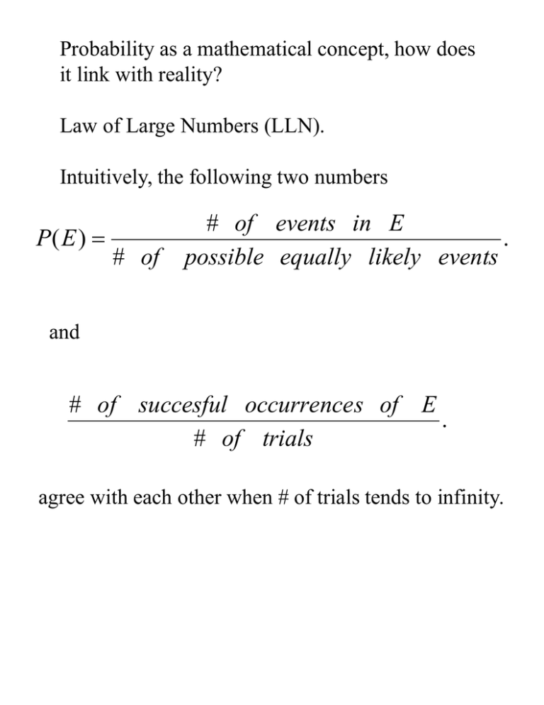
Intuitively, the following two numbers
P( E ) 
# of
# of events in E
.
possible equally likely events
and
# of succesful occurrences of E
.
# of trials
agree with each other when # of trials tends to infinity.
For example, consider rolling a dice: theoretically
(1 + 2 + 3 + 4 + 5 + 6) / 6 = 3.5.
In practice:
The Indian mathematician Brahmagupta (598–668) and
later the Italian mathematician Gerolamo Cardano
(1501–1576) stated without proof that the accuracies of
empirical statistics tend to improve with the number of
trials. This was then formalized as a law of large
numbers (LLN).
The LLN was first proved by Jacob Bernoulli.
It took him over 20 years to develop a sufficiently
rigorous mathematical proof which was published in
his Ars Conjectandi (The Art of Conjecturing) in 1713.
He named this his "Golden Theorem" .
In 1835, S.D. Poisson further described it under the
name "La loi des grands nombres" ("The law of large
numbers").
After Bernoulli and Poisson published their efforts,
other mathematicians also contributed to refinement of
the law, including Chebyshev, Markov, Borel, Cantelli
and Kolmogorov.
Who relies in the law of big numbers?
Who don’t?
Gambler’s fallacy.
While a run of five heads is only 1 in 32
(0.03125), it is 1 in 32 before the coin is first
tossed. After the first four tosses the results
are no longer unknown, so they do not count.
Reasoning that it is more likely that the next
toss will be a tail than a head due to the past
tosses—that a run of luck in the past
somehow influences the odds in the future—
is the fallacy.
A joke told among mathematicians
demonstrates the nature of the fallacy.
When flying on an aircraft, a man decides
always to bring a bomb with him. "The
chances of an aircraft having a bomb on it
are very small," he reasons, "and certainly
the chances of having two are almost
none!"
High Risk Little Gain?
P( not E ) * ( 1)
 P( E ) * G
0
Balance Condition.
P( not E )
G 
.
P( E )
Any payoff R : 1 with R < G
would not be fair. Indeed,
P( not E ) * ( 1)  P( E ) * R  0
if
R  G.
The expectation for the event E is
defined by
X ( E )  P( not E ) * ( 1)  P ( E ) * R.
In the above, the House Odd (or payoff for the player)
is given by
R : 1.
R represents the amount a player wins on a $1 bet (i.e.,
R + 1 in return, where 1 is the amount the player put
down).
Roulette–
the arts on
balancing
payoffs.
Bet name
Winning spaces
Payout
Odds against
winning
Expected value
(on a $1 bet)
0
0
35 to 1
37 to 1
−$0.053
00
00
35 to 1
37 to 1
−$0.053
Straight up
Any single number
35 to 1
37 to 1
−$0.053
Row 00
0, 00
17 to 1
18 to 1
−$0.053
Split
any two adjoining
numbers vertical or
horizontal
17 to 1
18 to 1
−$0.053
Trio
0, 1, 2 or 00, 2, 3
11 to 1
11.667 to 1
−$0.053
Street
any three numbers
horizontal (1, 2, 3
or 4, 5, 6 etc.)
11 to 1
11.667 to 1
−$0.053
Corner
any four adjoining
numbers in a block
(1, 2, 4, 5 or 17, 18,
20, 21 etc. )
8 to 1
8.5 to 1
−$0.053
Five Number Bet
0, 00, 1, 2, 3
6 to 1
6.6 to 1
−$0.079
Six Line
any six numbers
from two horizontal
rows (1, 2, 3, 4, 5, 6
or 28, 29, 30, 31,
32, 33 etc.)
5 to 1
5.33 to 1
−$0.053
1st Column
1, 4, 7, 10, 13, 16,
19, 22, 25, 28, 31,
34
2 to 1
2.167 to 1
−$0.053
2nd Column
2, 5, 8, 11, 14, 17,
20, 23, 26, 29, 32,
35
2 to 1
2.167 to 1
−$0.053
3rd Column
3, 6, 9, 12, 15, 18,
21, 24, 27, 30, 33,
36
2 to 1
2.167 to 1
−$0.053
1st Dozen
1 through 12
2 to 1
2.167 to 1
−$0.053
2nd Dozen
13 through 24
2 to 1
2.167 to 1
−$0.053
3rd Dozen
25 through 36
2 to 1
2.167 to 1
−$0.053
Odd
1, 3, 5, ..., 35
1 to 1
1.111 to 1
−$0.053
Even
2, 4, 6, ..., 36
1 to 1
1.111 to 1
−$0.053
, , ,
,
Red
1, 3, 5, 7, 9, 12,
14, 16, 18, 19, 21,
23,
25, 27, 30, 32, 34,
36
1 to 1
1.111 to 1
−$0.053
Black
2, 4, 6, 8, 10, 11,
13, 15, 17, 20, 22,
24,
26, 28, 29, 31, 33,
35
1 to 1
1.111 to 1
−$0.053
1 to 18
1, 2, 3, ..., 18
1 to 1
1.111 to 1
−$0.053
19 to 36
19, 20, 21, ..., 36
1 to 1
1.111 to 1
−$0.053
Example. Consider the following betting:
Amount
Betted  1
2
1



``0" ,   , ``1, 2, 3, 4, 5, 6" ,   , ``even"

House  R  35

R5

R 1
Odd R:1
Denote the expectation of the above betting by
X (1: 2 : 1; [4])
Here the numbers 1:2:1 recall the betting pattern,
and [4] denotes the total unit wagered ( = 4 unit).
The expectation of the above betting per unit is
given by
1
X (1: 2 : 1; [1])   X (1: 2 : 1; [4]).
4
Let us separate the
winning cases:
``0"
``1, 3, 5, "
``2, 3, 6, "
``6, 8, 10,, 30 32, 34, 36"


18  3  15


X (1: 2 : 1; [4])
1
(win on ``0", loss the other two)
 35  2 1
38 3
 5  2 1 1 (win on ``six", loss the other two)
-38
3
 5  2  1 --1 (win on ``six" and ``even", loss ``0" )
38
15
 1 1  2 (win on ``even", loss the other two)
38 -38 22
--1  2 1 (loss all three)

38
1
  35 
38 6
  5 2
38
18
 1 
38
37
 (1) 
38 -32

 (2) 
38
20
 (1)
38
That is,
X (1: 2 : 1; [4])
 X (``0"; [1])  2  X (``1,2,3,4,5,6"; [1])  X (``even"; [1])
 (0.053)  2  (0.053)  (0.053) .
Therefore,
1
X (1: 2 : 1; [1])   X (1: 2 : 1; [4])
4
  0.053 .
C
AC
A
B
WithoutA
Ao
AB
Note that the positions of
A, B, and C are “symmetric”.
Thus we focus on one of them,
say, A.
Bo
ABC
In the three events labelled A, B, and C as shown
above, one unit each is betted on each event:
1 : 1 : 1.
The returns (profits) are
RA , RB , and RC , respective ly.
Co
X (1:1:1; [3])
 P( Ao )  RA 1 1



-P( A )  R  R
-P( A )  R  R
-P( A )  R  R
-B
A
B
C
A
C
BC
A
1
1
 RC 
B
(win on ``A ", loss the other two)
(win on ``A " & ``B", loss on ``C")
(win on ``A " & ``C", loss on ``B")
(win on ``A ", ``B" & ``C")
 P(Bo )  RB 1A 1
-P(Without A)- R
(win on ``B ", loss the other two)
 P(Co )  RB 1A 1

B
 RC 1A 
--
(win on ``C ", loss the other two)
(win on ``B " & ``C", loss on ``A")
 { 1  [P( Ao )  P( AB )  P( AC )  P( ABC )  P(Bo )  P(Co )  P(Without A) } 1A 11
--
 RA [P( Ao )  P( AB )  P( AC )  P( ABC )]  (1A ) [P(Bo )  P(Co )  P(Without A)]
 1A  { 1  [P( Ao )  P( AB )  P( AC )  P( ABC )  P(Bo )  P(Co )  P(Without A)]}
up" to be A
"add

 

 other terms....
 RA  P( A)  (1A ) [P(Bo )  P(Co )  P(Without A)]
 1A  { [1  P( A)]  [P(Bo )  P(Co )  P(Without A)] }
 other terms....
 RA  P( A)
 1A  [1  P( A)]
 other terms....
 (1A ) [P(Bo )  P(Co )  P(Without A)]
 1A *[P(Bo )  P(Co )  P(Without A) ]
 (1) *(1)  1
 X ( A; [1])  other terms....
 X ( A; [1])  X (B; [1])  X (C; [1])
(via
 (convince youselves or
symmetry ).
heck the above for
B or C )
Nevertheless, the numerous even-money bets in
roulette have inspired many players over the years to
attempt to beat the game by using one or more
variations of a Martingale betting strategy, wherein
the gamer doubles the bet after every loss, so that the
first win would recover all previous losses, plus win a
profit equal to the original bet. This betting strategy is
fundamentally flawed in practice and the nearuniversal long-term consequence is a large financial
loss.
Another strategy is the Fibonacci system, where bets
are calculated according to the Fibonacci sequence.
1
2
3
5 8
13 21
1
Lose – go to the next Fibonacci number
Win - go back two steps until the first Fibonacci
number is reached.
Win the bet with the the first Fibonacci number, and
make a profit of $1.
In probability theory, the probability P of
some event E, denoted P(E), is usually
defined in such a way that P satisfies the
Kolmogorov axioms:
P ( E )  0.
(1)
( 2)
(3)
events )  1.
P(all
E1 , E2
then
be
mutually exclusive,
P( E1  E2 )  P ( E1 )  P( E2 ).
As
a
consequence,
P( E  [not E ])  P( all possibilities )  1
P( E1  [not E ])  P ( E1 )  P ( not E )
 P( E )  P( not E )  1
 P( not E )  1  P ( E ).
Show the following.
Suppose there are countable (finite) number of
events, separated from one another, and each one
has equal likelihood, then (roughly speaking)
P 
# of events in your favour
.
total # of events