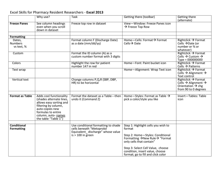
Excel Skills for Pharmacy Resident Researchers - Excel 2013
Freeze Panes
Why use?
Task
Getting there (toolbar)
See column headings
even when you scroll
down in dataset
Freeze top row in dataset
View—Window: Freeze Panes icon
 Freeze Top Row
Format column F (Discharge Date)
as a date (mm/dd/yy)
Home—Cells: Format Format
Cells Date
Formatting
Dates,
Numbers
vs text, %
Custom
Format the ID column (A) as a
custom number format with 3 digits
Colors
Highlight the row for patient
number 147 in red
Text wrap
Home—Alignment: Wrap Text icon
Vertical text
Format as Table
Conditional
Formatting
Home—Font: Paint bucket icon
Change columns P,Q,R (SBP, DBP,
HR) to be horizontal
Adds cool functionality
(shades alternate lines,
allows easy sorting and
filtering by column,
auto-copies new
formulas to entire
column, auto- names
the table “Table 1”)
Format the dataset as a Table---then Home—Styles: Format as Table 
undo it (Command Z)
pick a color/style you like
Use conditional formatting to shade
cells beneath “Metoprolol
Equivalent_ discharge” whose value
is > 100 in green
Step 1: Highlight cells you wish to
format
Step 2: Home—Styles: Conditional
Formatting New Rule “Format
only cells that contain”
Step 3: Select Cell Value, choose
condition, insert value, choose
format; go to fill and click color
Getting there
(alternate)
Rightclick  Format
Cells Date (or
number or % or
whatever)
Rightclick  Format
Cells  Custom 
Type = 000000000
Rightclick  Format
Cells  Patterns
Rightclick  Format
Cells  Alignment 
Text control
Rightclick  Format
Cells  Alignment 
Orientation  chg
from 90 to 0 degrees
Insert—Tables: Table
icon
Data Validation
Drop-down list
Ensures consistency of
data entry
Reduces risk of data
entry errors
Minimizes data
‘scrubbing’
Streamlines data
analysis
Create a column after “HF Clinic
Duration” for “Smoking_Status”
with the following choices: current,
past, never
Only numbers
**If you put text in a
numeric field, it can no
longer be read as a
numeric value!
Change columns “SBP” and “DBP” to Data—Data Tools: Data Validation
only allow numbers
icon  Data Validation  Allow:
Whole number OR decimal
Comment fields
Useful for verification
of outcomes by a
second chart reviewer
Use sparingly!
Functions
SUM
AVERAGE
COUNT
Numbers
MAX
MIN
Mathematical
functions
NOTE: Can add to the list later if
needed, just check the box “Apply
these changes to all other cells with the
same settings”
Calculate the mean, maximum and
minimum age
COUNTIF
Useful for counting
categorical data
IF (if/then)
Logic statement to
examine contents of a
cell, and if it meets
specific criteria, enter
something specific in
another cell.
Can create categories
or identify values that
Right click insert new column
Data  Data Tools: Data Validation
icon  Data Validation  Allow:
List, Source: type options
Formulas—Function Library: can find
function categories in library or
Insert Function icon  dialog box
with ALL Excel functions
For the column “HF Clinic Duration”,
have Excel calculate the number of
days each patient was enrolled in
the HF clinic
Count the number of females in this Formulas—Function Library: Insert
sample
Function icon  COUNTIF dialog
box select range  enter criteria
in quotes
Insert a column after
“BL_EF_actual” called “LVSD_BL”
that displays a value of 1 if the
patient has LVSD (that is, their
ejection fraction is <40%), 0 if they
do not, and be blank if an ejection
fraction is not available.
(formula is below)*
Formulas—Function Library: Insert
Function icon OR Logical icon  IF
dialog box
HINT: depict missing as “” and check
this first
Home  Editing  ∑
drop down
OR
Home  type in box “=
average”
are or are not in a
specified range
TTEST
Test for statistical
differences for a
continuous variable
CHISQUARE
VLOOKUP
Ex1=compare age in COPD vs nonCOPD patients
Ex2= Calculate the p value
comparing metoprolol equivalent
doses for baseline versus discharge
Compare the number of females vs
males in each group
Allows you to merge
datasets via a linking
variable (such as
patient medical record
number)
Insert a column after the one you
just created (LVSD_BL) that includes
the discharge EF data available in
Sheet1
Formulas—Function Library: Insert
Function icon  T.TEST dialog box
Arrays 1 and 2 are the ranges you
want to compare; tails usually =2;
type is usually 2
WEB:
http://www.graphpad.com/quickcalc
s/contingency1.cfm
Step 1: Name the “lookup” dataset:
Highlight cell range to name, then-Formulas—Defined Names: Name
Manager icon  New  Name table
name  Refers to cell range  OK
NOTE: Index variable (e.g. MRN) must be
in the 1st column of the named range
Step 2: Merge the “parent” and
“lookup” datasets:
Formulas—Function Library: Insert
Function icon  VLOOKUP dialog
box
Lookup_value is the linking variable
in your current dataset
Table_array is the dataset you are
looking in that has the linking
variable in the first column
Col_index_number tells you home
many columns over from the first
one to find the data element you
want
Range_lookup: type “FALSE” for an
exact match to the linking variable
Rightclick  Define
Name  then proceed
as per Name Manager
Pivot Tables
Can summarize large
amounts of data
Identify trends in data
for potential further
analysis
Eliminate duplicate IDs
* =IF(H3 ="","",IF(H3<40,1,0))
Ex1=Display gender by COPD status
in a NEW worksheet named
“Tables”
Ex2=Display mean metoprolol
Equivalent dose at discharge by
COPD status in the “Tables”
worksheet
Ex3=Display mean SBP by beta
blocker agent at discharge in the
“Tables” worksheet; Then limit to
just patients receiving metoprolol
Insert—Tables: PivotTable icon 
PivotTable
1. Confirm the cell range Excel
chooses
2. Choose location as new or existing
worksheet
3. drag fields to column labels
(groups), row labels (variables of
interest), and values boxes (data of
interest) below